Face Recognition: Traditional Approaches
Face Recognition for Human-Computer Interaction (HCI)
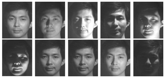
Main Problem
The variations between the images of the same face due to illumination and viewing direction are almost always larger than image variations due to change in face identity.
– Moses, Adini, Ullman, ECCV‘94
Closed Set vs. Open Set Identification
- Closed-Set Identification
- The system reports which person from the gallery is shown on the test image: Who is he?
- Performance metric: Correct identification rate
- Open-Set Identification
- The system first decides whether the person on the test image is a known or unknown person. If he is a known person who he is?
- Performance metric
- False accept: The invalid identity is accepted as one of the individuals in the database.
- False reject: An individual is rejected even though he/she is present in the database.
- False classify: An individual in the database is correctly accepted but misclassified as one of the other individuals in the training data
Authentication/Verification
A person claims to be a particular member. The system decides if the test image and the training image is the same person: Is he who he claims he is?
Performance metric:
- False Reject Rate (FRR): Rate of rejecting a valid identity
- False Accept Rate (FAR): Rate of incorrectly accepting an invalid identity.
Feature-based (Geometrical) approaches
“Face Recognition: Features versus Templates” 1
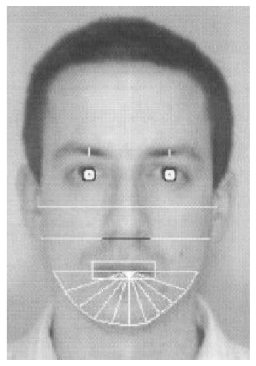
- Eyebrow thickness and vertical position at the eye center position
- A coarse description of the left eyebrow‘s arches
- Nose vertical position and width
- Mouth vertical position, width, height upper and lower lips
- Eleven radii describing the chin shape
- Face width at nose position
- Face width halfway between nose tip and eyes
Classification
Nearest neighbor classifier with Mahalanobis distance as the distance metric: $$ \Delta_{j}(x)=\left(x-m_{j}\right)^{T} \Sigma^{-1}\left(x-m_{j}\right) $$
- $x$: input face image
- $m_j$: average vector representing the $j$-th person
- $\Sigma$: Covariance matrix
Different people are characterized only by their average feature vector.
The distribution is common and estimated by using all the examples in the training set.
Appearance-based approaches
Can be either
- holistic (process the whole face as the input), or
- local / fiducial (process facial features, such as eyes, mouth, etc. seperately)
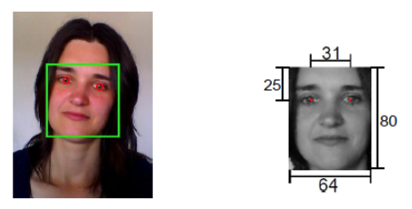
Processing steps: align faces with facial landmarks
- Use manually labeled or automatically detected eye centers
- Normalize face images to a common coordination, remove translation,, rotation and scaling factors
- Crop off unnecessary background
Holistic appearance-based approaches
Eigenfaces
💡 Idea
A face image defines a point in the high dimensional image space.
Different face images share a number of similarities with each other
- They can be described by a relatively low dimensional subspace
- Project the face images into an appropriately chosen subspace and perform classification by similarity computation (distance, angle)
- Dimensionality reduction procedure used here is called Karhunen-Loéve transformation or principal component analysis (PCA)
Objective
Find the vectors that best account for the distribution of face images within the entire image space
PCA
For more details see: Principle Component Analysis (PCA)
- Find direction vectors so as to minimize the average projection error
- Project on the linear subspace spanned by these vectors
- Use covariance matrix to find these direction vectors
- Project on the largest K direction vectors to reduce dimensionality
PCA for eigenfaces:
$y$: Face image
$Y$: Face matrix
$m$: Mean face
$C$: Covariance matrix
$D$: Eigenvalues
$U$: Eigenvectors
$\Omega$: Representation coefficients
Training
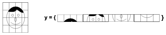
Acquire initial set of face images (training set): $$ Y = [y_1, y_2, \dots, y_K] $$
Calculate the eigenfaces/eigenvectors from the training set, keeping only the $M$ images/vectors corresponding to the highest eigenvalues $$ U = (u_1, u_2, \dots, u_M) $$
Calculate representation of each known individual $k$ in face space $$ \Omega_k = U^T(y_k - m) $$
Testing
Project input new image y into face space $$ \Omega = U^T(y - m) $$
Find most likely candidate class $k$ by distance computation $$ \epsilon_k = \|\Omega - \Omega_k\| \quad \text{for all } \Omega_k $$
Projections onto the face space
Principal components are called “eigenfaces” and they span the “face space”.
Images can be reconstructed by their projections in face space:
$$ Y_f = \sum_{i=1}^{M} \omega_i u_i $$
Appearance of faces in face-space does not change a lot
Difference of mean-adjusted image $(Y-m)$ and projection $Y_f$ gives a measure of „faceness“
- Distance from face space can be used to detect faces
Different cases of projections onto face space
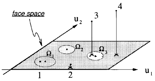
Case 1: Projection of a known individual
$\rightarrow$ Near face space ($\epsilon < \theta_{\delta}$) and near known face $\Omega_k$ ($\epsilon_k < \theta_{\epsilon}$)
Case 2: Projection of an unkown individual
$\rightarrow$ Near face space, far from reference vectors
Case 3 and 4: not a face (far from face space)
PCA for face matching and recognition
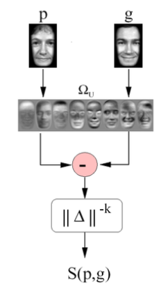
- Projects all faces onto a universal eigenspace to “encode” via principal components
- Uses inverse-distance as a similarity measure $S(p,g)$ for matching & recognition
Problems and shortcomings
Eigenfaces do NOT distinguish between shape and appearance
PCA does NOT use class information
- PCA projections are optimal for reconstruction from a low dimensional basis, they may not be optimal from a discrimination standpoint
Fisherface
Linear Discriminant Analysis (LDA)
For more details about LDA, see: LDA Summary)
- A.k.a. Fischer‘s Linear Discriminant
- Preserves separability of classes
- Maximizes ratio of projected between-classes to projected within-class scatter
$$ W_{\mathrm{fld}}=\arg \underset{W}{\max } \frac{\left|W^{T} S_{B} W\right|}{\left|W^{T} S_{W} W\right|} $$
Where
- $S_{B}=\sum_{i=1}^{c}\left|x_{i}\right|\left(\mu_{i}-\mu\right)\left(\mu_{i}-\mu\right)^{T}$: Between-class scatter
- $c$: Number of classes
- $\mu_i$: mean of class $X_i$
- $|X_i|$: number of samples of $X_i$
- $S_{W}=\sum_{i=1}^{c} \sum_{x_{k} \in X_{i}}\left(x_{k}-\mu_{i}\right)\left(x_{k}-\mu_{i}\right)^{T}$: Within-class scatter
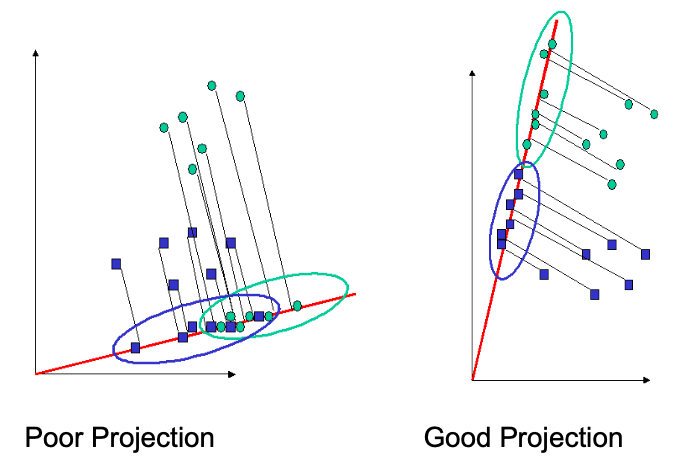
LDA vs. PCA
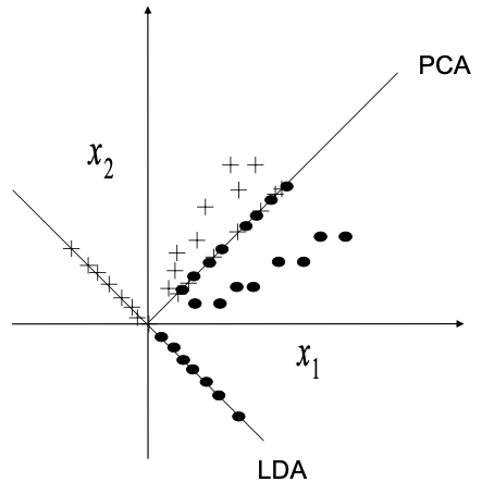
LDA for Fisherfaces
Fisher’s Linear Discriminant
- projects away the within-class variation (lighting, expressions) found in training set
- preserves the separability of the classes.
Local appearance-based approach
Local vs Holistic approaches:
- Local variations on the facial appearance (different expression,occlsion, lighting)
- lead to modifications on the entire representation in the holistic approaches
- while in local approaches ONLY the corresponding local region is effected
- Face images contain different statistical illumination (high frequency at the edges and low frequency at smooth regions). It’s easier to represent the varying statistics linearly by using local representation.
- Local approaches facilitate the weighting of each local region in terms of their effect on face recognition.
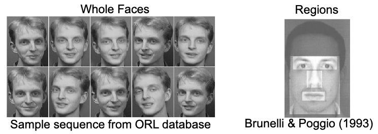
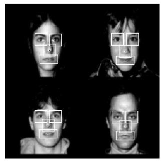
Modular Eigen Spaces
Classification using fiducial regions instead of using entire face 2.
Local PCA (Modular PCA)
Face images are divided into $N$ smaller sub-images
PCA is applied on each of these sub-images
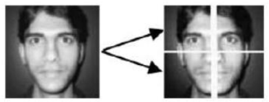
Performed better than global PCA on large variations of illumination and expression
No imporvements under variation of pose
Local Feature based
🎯 Objective: To mitigate the effect of expression, illumination, and occlusion variations by performing local analysis and by fusing the outputs of extracted local features at the feature or at the decision level.
Gabor Filters
Elastic Bunch Graphs (EBG)
Local Binary Pattern (LBP) Histogram
http://cbcl.mit.edu/people/poggio/journals/brunelli-poggio-IEEE-PAMI-1993.pdf ↩︎
Pentland, Moghaddam and Starner, “View-based and modular eigenspaces for face recognition,” 1994 Proceedings of IEEE Conference on Computer Vision and Pattern Recognition, Seattle, WA, USA, 1994, pp. 84-91, doi: 10.1109/CVPR.1994.323814. ↩︎