People Detection: Part-based Approaches

Motivation

• Model body-parts separately
• Break down an objects’ overall variability into more manageable pieces
• Pieces can be classified by less complex classifiers
• Apply prior knowledge by (manually) splitting the global object into meaningful parts
• Advantages
  • deal better with moving body parts (poses)
  • able to handle occlusions, overlaps
  • sharing of training data
• Disadvantages
  • require more complex reasoning
  • problems with low resolutions

Part-based models

• Two main components

  • parts (2D image fragments)

  • structure (configuration of parts) $\rightarrow$ often also part-combination method

    • Fixed spatial layout

      • Local parts are modeled to have a mostly fixed position and orientation with respect to the object or detection window center

    • Flexible Spatial Layout

      • local parts are allowed to shift in location and scale
      • can better handle deformations or articulation changes
      • well suited for non-rigid objects
      • spatial relations are often modeled probabilistically

The Mohan People Detector ¹

• 4 parts
  • face and shoulder
  • legs
  • right arm
  • left arm
• Fixed layout
  • Body parts are not always at the exact same position
  • Allow local shifts: in position and in scale
  • Best location has to be found for each detection window
• Combination: Classifier (SVM)
• Detection
  • sliding window approach
  • 64x128 pixels

The Implicit Shape Model (ISM) ²

💡 Main ideas

• Automatically learn a large number of local parts that occur on the object (referred to as visual vocabulary, bag of words or codebook)
• Learn a star-topology structural model
  • features are considered independent given the objects’ center
  • likely relative positions are learned from data

5 steps

1. Part detection/localization
2. Part description
3. Learning part appearance
4. Learning theh spatial layout of parts
5. Combination of part detections

Part Detection/Localization

A good part decomposition needs to be

• Repeatable

  We should be able to find the part despite articulation or image transformations (e.g. invariance to rotation, perspective, lighting)

• Distinctive

  • A part should not be easily confused with other parts the regions should contain an “interesting” structure

• Compact

  No lengthy or strangely shaped parts

• Efficient

  Computationally inexpensive to detect or represent

• Cover

  Parts need to sufficiently cover the object

Local features

Two components of local features:

• key- or interest-points (“Where is it?”)
  • specify repeatable points on the object
  • consist of x-, y-position and scale
• local (keypoint) descriptors (“How does it look like?”)
  • describe the area around an interest point
  • i.e. define the feature representation of an interest point

General approach

• Find keypoints using keypoint detector
• Define region around keypoint
• Normalize region
• Compute local descriptor
• Compare descriptors

Keypoint detectors

Find reproducible, scale invariant local keypoints in an image

Keypoint Localization

• Goals
  • repeatable detection
  • precise localization
  • interesting content
• Idea: Look for two-dimensional signal changes

Hessian Detector

Search for strong second derivatives in two orthogonal directions (Hessian determinant) $$ \operatorname{Hessian}(I)=\left[\begin{array}{ll} I_{x x} & I_{x y} \\ I_{x y} & I_{y y} \end{array}\right] $$

$$ \operatorname{det}(\operatorname{Hessian}(I))=I_{x x} I_{y y}-I_{x y}^{2} $$

Second Partial Derivative Test: If $det(H)>0$, we have a local minimum or maximum.

Example:

Responses:

Handle scale

• Scale Space

  Not only detect a distinctive position, but also a characteristic scale around an interest point

  

• Scale Invariance

  • Same operator responses, if the patch contains the same image up to a scale factor

    

  • Automatic Scale Selection: Function responses for increasing scale (scale signature)

    • Laplacian-of-Gaussian (LoG)

      

Part Description

Distinctly describe local keypoints and achieve orientation invariance

Local Descriptors

• Goal: Describe (local) region around a keypoint
• Most available descriptors focus on edge/gradient information
  • Capture boundary and texture information
  • Color still used relatively seldom

Orientation Invariance

• Compute orientation histogram
• Select dominant orientation
• Normalize: rotate to fixed orientation

• The SIFT descriptor: Histogram of gradient orientations

  • captures important texture information

  • robust to small translations / affine deformations

  • How it works? (similar to HOG)

    
    • region rescaled to a grid of 16x16 pixels (8x8 in image)
    • 4x4 regions (2x2 in image) = 16 histograms (concatenated)
    • histograms: 8 orientation bins, gradients weighted by gradient magnitude
    • final descriptor has 128 dimensions and is normalized to compensate for illumination differences

A brief introduction: SIFT - 5 Minutes with Cyrill

A nice explanation: (source: https://gilscvblog.com/2013/08/18/a-short-introduction-to-descriptors/)

SIFT was presented in 1999 by David Lowe and includes both a keypoint detector and descriptor. SIFT is computed as follows:

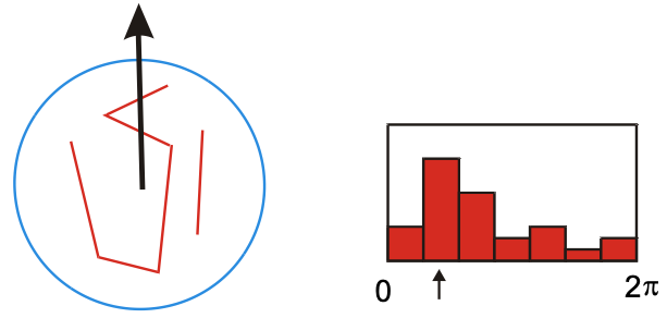
1. First, detect keypoints using the SIFT detector, which also detects scale and orientation of the keypoint.
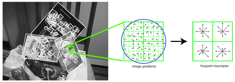
2. Next, for a given keypoint, warp the region around it to canonical orientation and scale and resize the region to 16X16 pixels.

3. Compute the gradients for each pixels (orientation and magnitude).

4. Divide the pixels into 16, 4X4 pixels squares.

5. For each square, compute gradient direction histogram over 8 directions

6. concatenate the histograms to obtain a 128 (16*8) dimensional feature vector:

SIFT descriptor illustration:

SIFT is invariant to illumination changes, as gradients are invariant to light intensity shift. It’s also somewhat invariant to rotation, as histograms do not contain any geometric information.

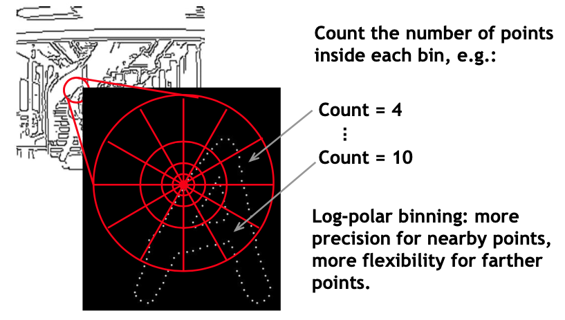
Shape Context Descriptor

What Local Features Should I Use?

• Best choice often application dependent
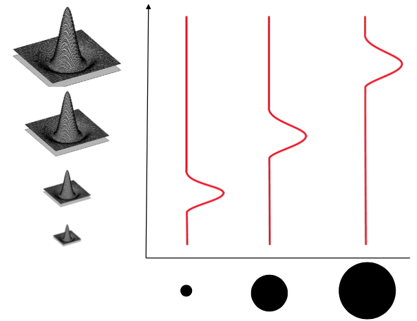
  • Harris-/Hessian-Laplace/DoG work well for many natural categories
• More features are better
  • combining several detectors often helps

Learning Part Appearances

Visual Vocabulary

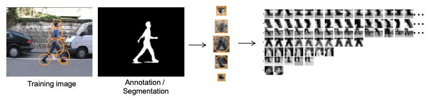
1. Detect keypoints on all person training examples
2. Compute local descriptors for all keypoints

-> Result: Large set of local image descriptors that all occur on people

Group visually similar local descriptors

• similar local descriptors = parts that are reoccurring

• parts, that occur only rarely are discarded (they could result from noise or background structures)

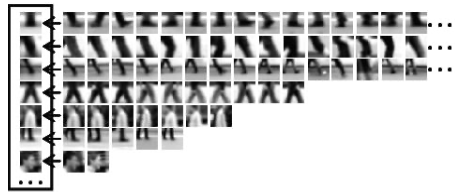
• result: descriptor groups representing human body parts

• Grouping Algorithms / Clustering

  • Partitional Clustering
    • K-Means
    • Gaussian Mixture Clustering (EM)
  • Hierarchical of Agglomerative Clustering
    • Single-Link (minimum)
    • Group-Average
    • Ward’s method (minimum variance)

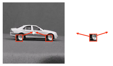
Learning the Spatial Layout of Parts

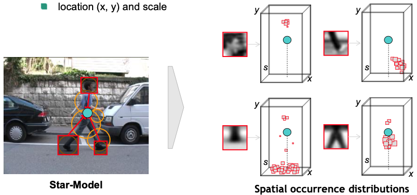
Spatial Occurrence (Star-Model)

• Record spatial occurrence

  • match vocabulary entries to training images

  • record occurrence distributions with respect to object center (location $(x, y)$ and scale)

    

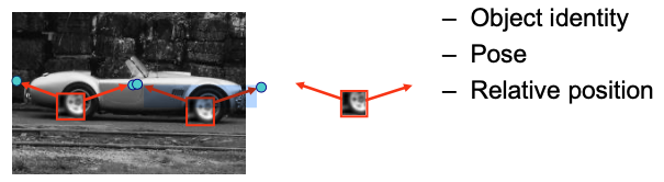
Generalized Hough Transform

• For every feature, store possible “occurrences”

  

• For new image, let the matched features vote for possible object positions

  

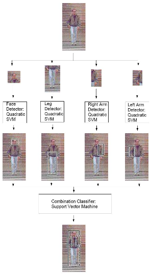
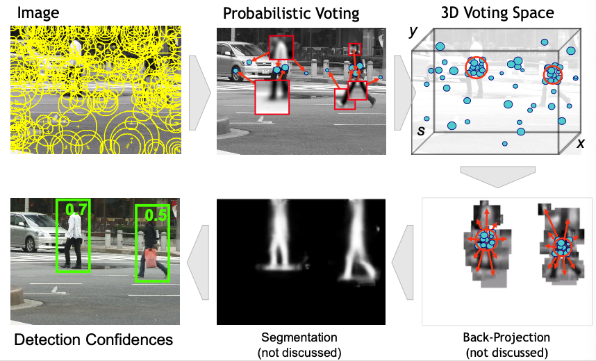
Combination of Part Detections

ISM Detection Procedure: