Tracking
Introduction
Tracking Vs. Detection
Detection: Find an object in a single image
- Face, person, body part, facial landmarks, …
- No assumption about dynamics, temporal consistency made
Tracking:
determine a target’s locations (and/or rotation, deformation, pose, …) over a sequence of images
i.e.: determine the target’s state (location and/or rotation, deformation, pose, …) over a sequence of observations derived from images
Provides object positions (etc.) in each frame
Motivation
- Use more than one image to analyse the scene
- Use a-priori knowledge to improve analysis
- system dynamics, imaging / measurment process,
Target types
- Single objects: face, person, …
- Multiple objects: group of people, head and hands, …
- Articulated body: full body, hand
Sensor setup
- Single camera
- Multiple cameras
- Active cameras
- Cameras + microphones
observations used for tracking
- Templates
- Color
- Foreground-Background segmentation Edges
- Dense Disparity
- Optical flow
- Detectors (body, body parts)
Tracking as State Estimation
- Want to predict state of the system (position, pose, …)
- But state cannot directly be measured
- Only certain observations (measurements) can be made
- But Observations are noisy! (due to measurement errors)
What is the most likely state $x$ of the system at a given time, given a sequence of observations $Z_t$ ? $$ \arg \max p\left(x_{t} \mid Z_{t}\right) $$
$x_t$: state of the system at time $t$
$z_t$: Observation / measurement about the certain aspects of the system at
time $t$
Observations up to time $t$: $z_{1:t}$ or $Z_t$
Bayes Filter
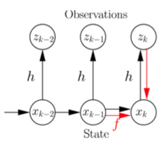
Assume state $x$ to be Markov process $$ p\left(x_{t} \mid x_{t-1}, x_{t-2}, . ., x_{0}\right)=p\left(x_{t} \mid x_{t-1}\right) $$
States $x$ generate observations $z$ $$ p\left(z_{t} \mid x_{t}, x_{t-1}, . ., x_{0}\right)=p\left(z_{t} \mid x_{t}\right) $$
Want to estimate most likely state $x_t$ given sequence $Z_t$: $$ \arg \max p\left(x_{t} \mid Z_{t}\right) $$
Can be estimated recursively
Need:
- Process model: $p(x_t | x_{t-1})$
- Measurement model: $p(z_t | x_t)$
Helpful resource:
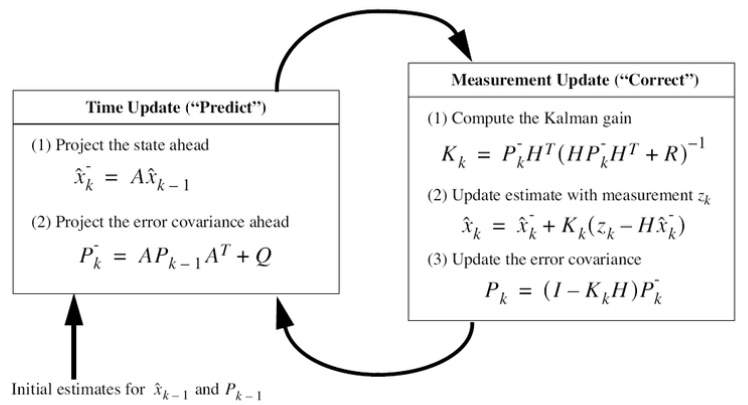
Kalman filter
- An instance of a Bayes filter
- Assumes
- Linear state propagation and measurement model
- Gaussian process and measurement noise
The process to be estimated: $$ \begin{array}{ll} x_{k}=A x_{k-1}+w_{k-1} & \quad p(w) \sim N(0, Q) \\ z_{k}=H x_{k}+v_{k} & \quad p(v) \sim N(0, R) \end{array} $$
- $x_k$: state at time $k$
- $A$: transition matrix
- $z_k$: obeservation at time $k$
- $H$: measurement matrix
- $p(w) \sim N(0, Q)$: process noise
- $p(v) \sim N(0, R)$: measurement noise
Note:
The simple Kalman Filter is NOT applicable, when the process to be estimated is NOT linear or the measurement relationship to the process is NOT linear.
$\rightarrow$ The Extended Kalman Filter (EKF) linearizes about the current mean and covariance
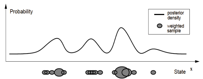
Paticle Filter
Helpful resources:
- The Kalman Filter often fails when the measurement density is multimodal / non-Gaussian.
- A Particle Filter represents and propagates arbitrary probability distributions. They are represented by a set of weighted samples.
- The Particle Filtering is a numerical technique (unlike the Kalman filter which is analytical).
- Like a Kalman Filter, a Particle Filter incorporates a dynamic model describing system dynamics
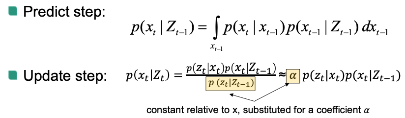
Bayesian Tracking
Bayes rule applied to tracking $$ \arg \max _{x_{t}} p\left(x_{t} \mid Z_{t}\right)=\arg \max _{x_{t}} p\left(z_{t} \mid x_{t}\right) p\left(x_{t} \mid Z_{t-1}\right) $$
$$ p\left(x_{t} \mid Z_{t-1}\right)=\int_{x_{t-1}} p\left(x_{t} \mid x_{t-1}\right) p\left(x_{t-1} \mid Z_{t-1}\right) $$
Simplifying assumption (Markov): $$ p\left(x_{t} \mid X_{t-1}\right)=p\left(x_{t} \mid x_{t-1}\right) $$ where
- $x_t$: state at time $t$
- $z_t$: observation at time $t$
- $X_t$: history of states up to the time $t$
- $Z_t$: history of observations up to $t$
Observation and Motion Model
- $p(z_t | x_t)$: The likelihood that the $z_t$ is observed, given that the true state of the system is represented by $x_t$
- $p(x_{t} | x_{t-1})$: The likelihood that the state of the system is $x_t$ when the previous state was $x_{t-1}$
Factored Sampling
Probability density function is represented by weighted samples (“particles“)
Particle Filter (PF)
For a PF tracker, you need
a set of $N$ weighted samples (particle) at time $k$ $$ \left\{\left(s_{k}^{(i)}, \pi_{k}^{(i)}\right) \mid i=1 \dots N\right\} $$
the motion model $$ s_{k}^{(i)} \leftarrow s_{k-1}^{(i)} $$
the observation model $$ \pi_{k}^{(i)} \leftarrow s_{k}^{(i)} $$
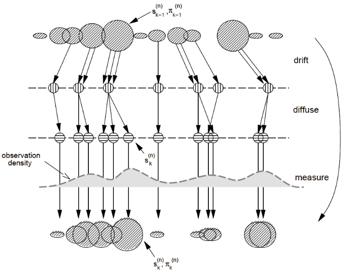
The Condensation Algorithm
A popular instance of a particle filter in Computer Vision
Select
Randomly select $N$ new samples $S_{k}^{(i)}$ from the old sample set $S_{k-1}^{(i)}$ according to their weights $\pi_{k-1}^{(i)}$
Predict
Propagate the samples using the motion model
Measure
Calculate weights for the new samples using the observation model $$ \pi_{k}^{(i)}=p\left(z_{k} \mid x_{k}=s_{k}^{(i)}\right) $$
Illustration:
How to get the target position?
- Cluster the particle set and search for the highest mode
- Just take the strongest particle
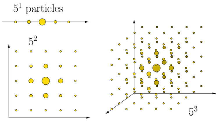
How many particles are needed?
- Depends strongly on the dimension of the state space!
- Tracking 1 object in the image plane typically requires 50-500 particles
Problem
The Dimensionality Problem
Examples
Tracking one Face with a Particle Filter
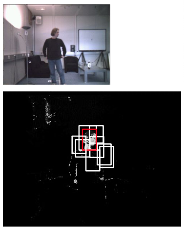
State: ($x$, $y$, scale)
Observations: skin color
Procedure:
Select and predict samples
Measurement step
For each particle
- Count supporting skin pixels in box defined by ($x$, $y$, scale)
- Particle weights determined based on skin color support
Particle with maximum weight choosen as best solution
Tracking multiple objects
Two different approaches:
- A dedicated tracker for each of the objects
- Start with one tracker, once an object is tracked, initialize one more tracker to search for more objects
- Typically fast and well parallelizable
- Optimal global assignment / tracking difficult to find, Information has to be shared across trackers to find a good assignment
- A single tracker in a joint state space
- Easier to find optimal assignment
- Number of objects has to be known in advance
- State space becomes high dimensional (curse of dimensionality)
Face and Head Pose Tracking
- Particle filter: Head-pose estimation integrated in the tracker
- Observation model
- Use bank of face detectors for different poses
- Update particle weights with score of matching detector, i.e. the detector with closest angle to hypothesis
- Dynamical model: Gaussian noise, no explicit velocity model
- Occlusion handling
- Set particle weight to zero, if it is too close to another track’s center