Histogram of Oriented Gradients (HOG)

What is a Feature Descriptor

A feature descriptor is a representation of an image or an image patch that simplifies the image by extracting useful information and throwing away extraneous information.

Typically, a feature descriptor converts an image of size $\text{width} \times \text{height} \times 3 \text{(channels)}$ to a feature vector / array of length $n$. In the case of the HOG feature descriptor, the input image is of size $64 \times 128 \times 3$ and the output feature vector is of length $3780$.

How to calculate Histogram of Oriented Gradients?

In this section, we will go into the details of calculating the HOG feature descriptor. To illustrate each step, we will use a patch of an image.

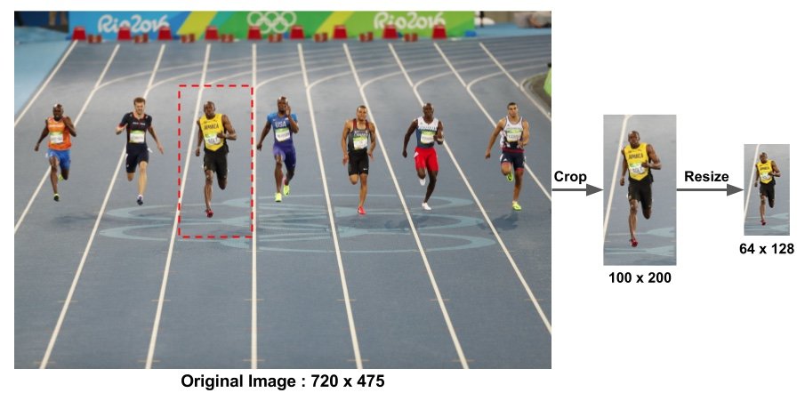
1. Preprocessing

Typically patches at multiple scales are analyzed at many image locations. The only constraint is that the patches being analyzed have a fixed aspect ratio.

In our case, the patches need to have an aspect ratio of 1:2. For example, they can be 100×200, 128×256, or 1000×2000 but not 101×205.

For the example image of size 720x475 below, we select a patch of size 100x200 for calculating HOG feature descriptor. This patch is then cropped out of an image and resized to 64×128.

2. Calculate the Gradient Images

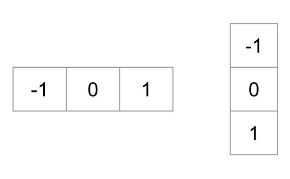
To calculate a HOG descriptor, we need to first calculate the horizontal and vertical gradients; after all, we want to calculate the histogram of gradients.

Calculating the horizontal and vertical gradients is easily achieved by filtering the image with the following kernels (Sobel operator).

Next, we can find the magnitude and direction of gradient using the following formula: $$ \begin{array}{l} g=\sqrt{g_{x}^{2}+g_{y}^{2}} \\ \theta=\arctan \frac{g_{y}}{g_{x}} \end{array} $$ The figure below shows the gradients:

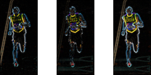
At every pixel, the gradient has a magnitude and a direction. For color images, the gradients of the three channels are evaluated ( as shown in the figure above ). The magnitude of gradient at a pixel is the maximum of the magnitude of gradients of the three channels, and the angle is the angle corresponding to the maximum gradient.

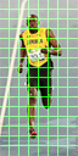
3. Calculate Histogram of Gradients in 8×8 cells

In this step, the image is divided into 8×8 cells and a histogram of gradients is calculated for each 8×8 cells.

Let’s look at one 8×8 patch in the image and see how the gradients look.

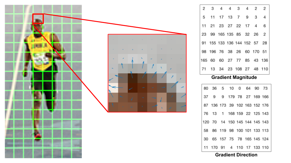
• The image in the center shows the patch of the image overlaid with arrows showing the gradient — the arrow shows the direction of gradient and its length shows the magnitude. The direction of arrows points to the direction of change in intensity and the magnitude shows how big the difference is.

• On the right, gradient direction is represented by angles between 0 and 180 degrees instead of 0 to 360 degrees. These are called “unsigned” gradients because a gradient and it’s negative are represented by the same numbers. Empirically it has been shown that unsigned gradients work better than signed gradients for pedestrian detection.

The next step is to create a histogram of gradients in these 8×8 cells. The histogram contains 9 bins corresponding to angles 0, 20, 40 … 160 of $y$-axis.

The following figure illustrates the process. We are looking at magnitude and direction of the gradient of the same 8×8 patch as in the previous figure. A bin is selected based on the direction, and the vote ( the value that goes into the bin ) is selected based on the magnitude.

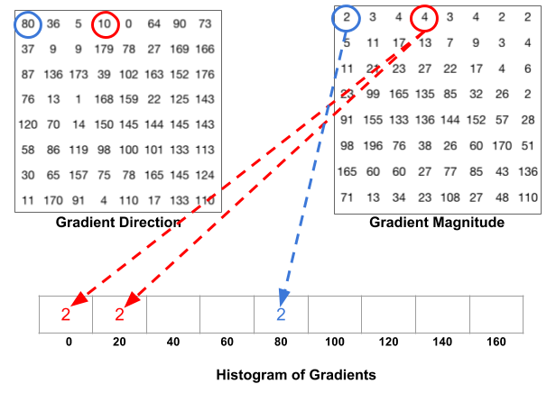
• For the pixel encircled in blue: It has an angle ( direction ) of 80 degrees and magnitude of 2. So it adds 2 to the 5th bin (bin for angle 80).
• For the pixel encircled in red: It has an angle of 10 degrees and magnitude of 4. Since 10 degrees is half way between 0 and 20, the vote by the pixel splits evenly into the two bins.

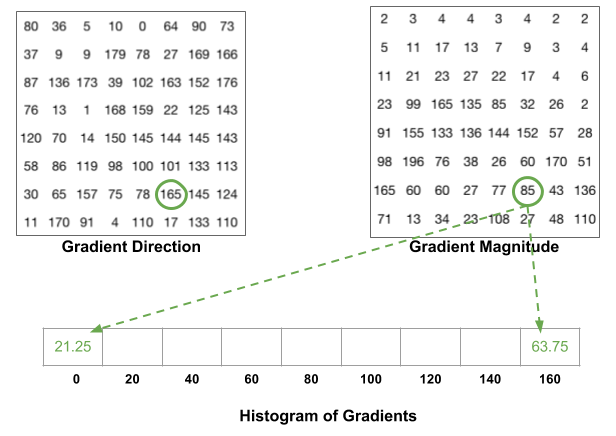
One more detail to be aware of: If the angle is greater than 160 degrees, it is between 160 and 180, and we know the angle wraps around making 0 and 180 equivalent. So in the example below, the pixel with angle 165 degrees contributes proportionally to the 0 degree bin and the 160 degree bin.

The contributions of all the pixels in the 8×8 cells are added up to create the 9-bin histogram. For the patch above, it looks like this

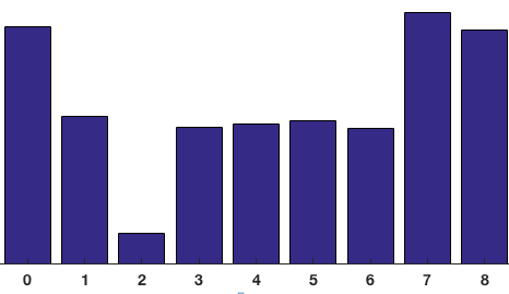
As aforementioned, the $y$-axis is 0 degrees. We can see the histogram has a lot of weight near 0 and 180 degrees, which is just another way of saying that in the patch gradients are pointing either up or down.

4. 16×16 Block Normalization

In the last step, we created a histogram based on the gradient of the image. However, gradients of an image are sensitive to overall lighting. Ideally, we want our descriptor to be independent of lighting variations. In other words, we would like to “normalize” the histogram so they are not affected by lighting variations.

Instead of normalizing just a single 8x8 cell, we’ll normalize over a bigger sized block of 16×16. A 16×16 block has 4 histograms which can be concatenated to form a 36 x 1 element vector. The window is then moved by 8 pixels (see animation) and a normalized 36×1 vector is calculated over this window and the process is repeated.

5. Calculate the HOG feature vector

To calculate the final feature vector for the entire image patch, the 36×1 vectors are concatenated into one giant vector:

• Number of 16x16 blocks: $7 \times 15 = 105$
• Each 16x16 block is represented by a $36\times1$ vector

Therefore, the giant vector has the dimension $36 \times 105 = 3780$

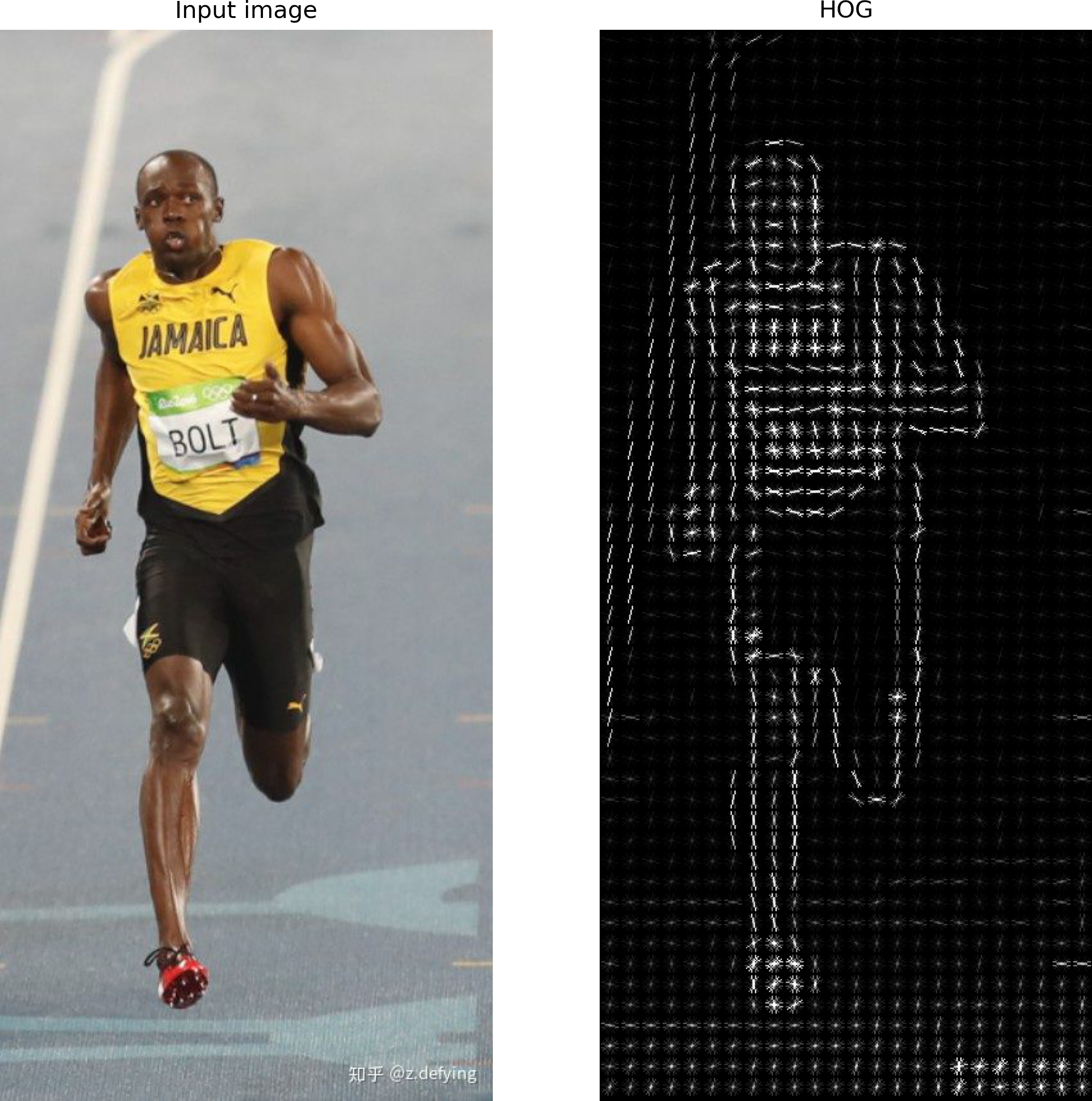
HOG visualization

from skimage import io
from skimage.feature import hog
from skimage import data, exposure
from google.colab.patches import cv2_imshow
import matplotlib.pyplot as plt

image = io.imread('https://pic4.zhimg.com/80/v2-2ccc671e60031942dca8a129410a0383_720w.jpg')

fd, hog_image = hog(image, orientations=8, pixels_per_cell=(16, 16),
                    cells_per_block=(1, 1), visualize=True, multichannel=True)

fig, (ax1, ax2) = plt.subplots(1, 2, figsize=(10, 10), sharex=True, sharey=True)
ax1.axis('off')
ax1.imshow(image, cmap=plt.cm.gray)
ax1.set_title('Input image')

# Rescale histogram for better display
hog_image_rescaled = exposure.rescale_intensity(hog_image, in_range=(0, 10))
ax2.axis('off')
ax2.imshow(hog_image_rescaled, cmap=plt.cm.gray)
ax2.set_title('HOG')

plt.show()

Reference

• Histogram of Oriented Gradients: clear and detailed explanation 👍
• HOG特征详解: HOG visualization
• Video explanation: