Overview of Region-based Object Detectors

Sliding-window detectors

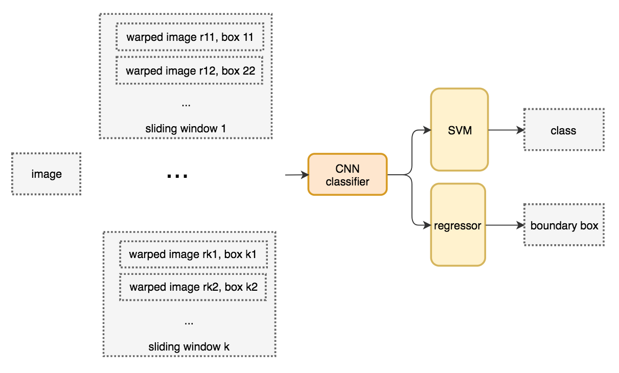
A brute force approach for object detection is to slide windows from left and right, and from up to down to identify objects using classification. To detect different object types at various viewing distances, we use windows of varied sizes and aspect ratios.

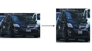
We cut out patches from the picture according to the sliding windows. The patches are warped since many classifiers take fixed size images only.

The warped image patch is fed into a CNN classifier to extract 4096 features. Then we apply a SVM classifier to identify the class and another linear regressor for the boundary box.

System flow:

Pseudo-code:

for window in windows:
    patch = get_patch(image, window)
    results = detector(patch)

We create many windows to detect different object shapes at different locations. To improve performance, one obvious solution is to reduce the number of windows.

Selective Search

Instead of a brute force approach, we use a region proposal method to create regions of interest (ROIs) for object detection.

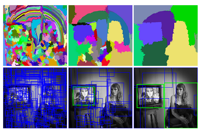
In selective search (SS)

1. We start with each individual pixel as its own group
2. We calculate the texture for each group and combine two that are the closest ( to avoid a single region in gobbling others, we prefer grouping smaller group first).
3. We continue merging regions until everything is combined together.

The figure below illustrates this process:

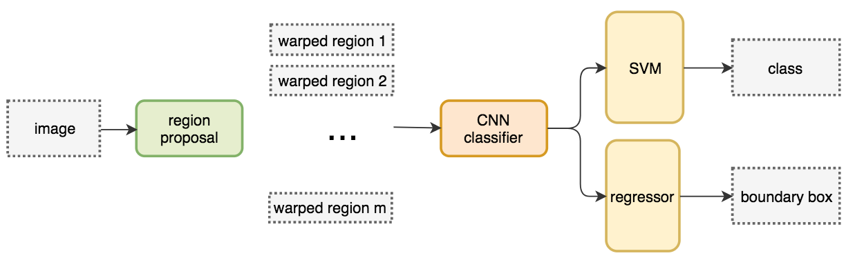
R-CNN ¹

Region-based Convolutional Neural Networks (R-CNN )

1. Uses of a region proposal method to create about 2000 ROIs (regions of interest).
2. The regions are warped into fixed size images and feed into a CNN network individually.
3. Uses fully connected layers to classify the object and to refine the boundary box.

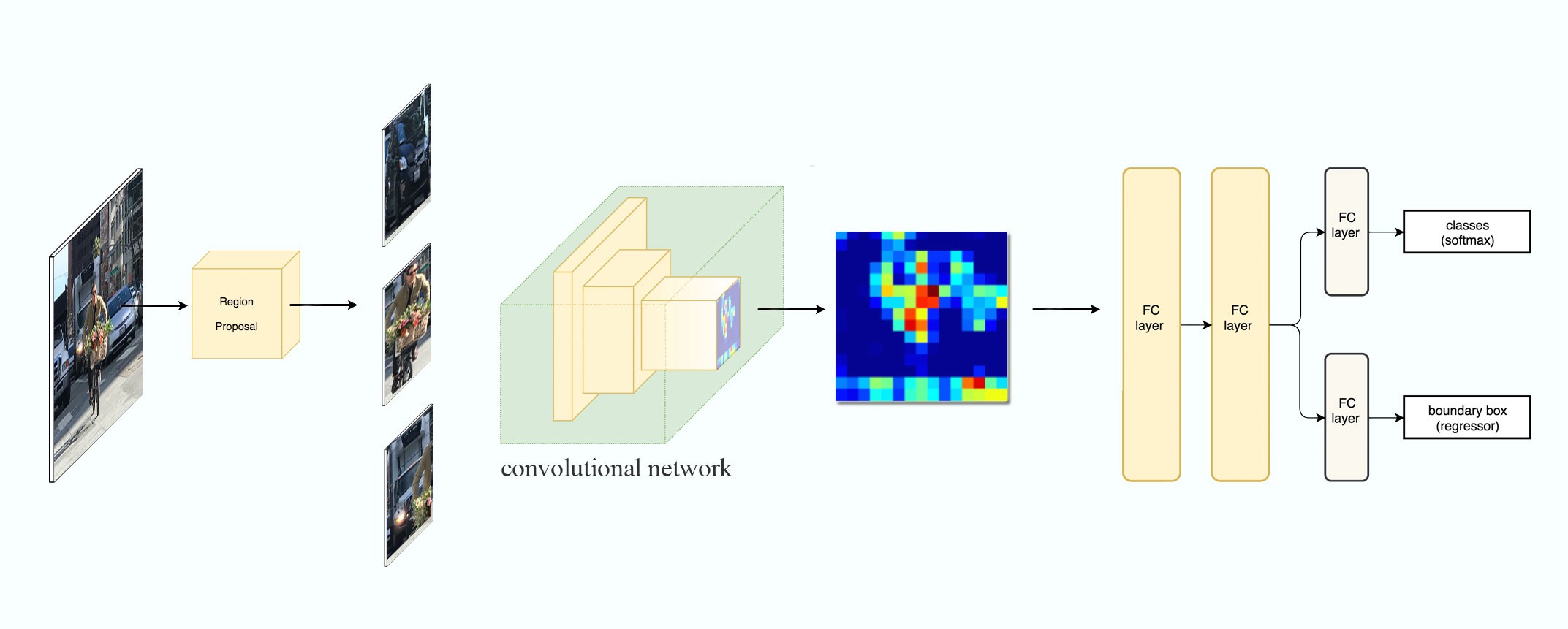
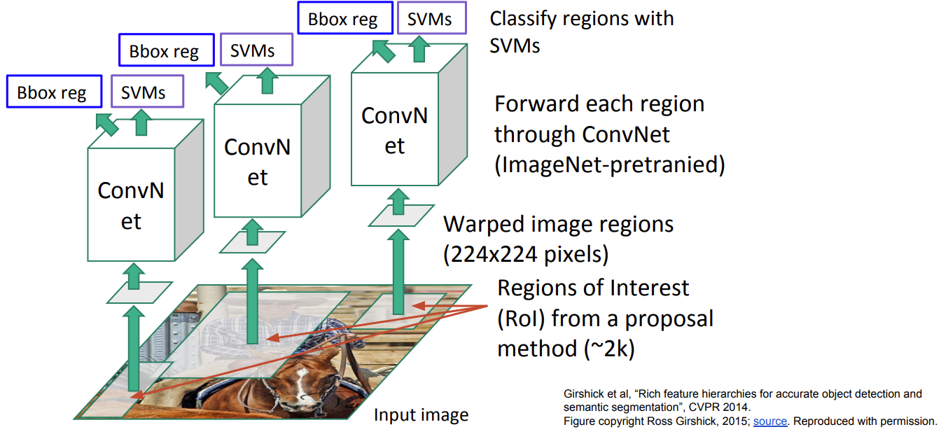
System flow:

Pseudo-code:

ROIs = region_proposal(image) # RoI from a proposal method (~2k)
for ROI in ROIs:
    patch = get_patch(image, ROI)
    results = detector(patch)

With far fewer but higher quality ROIs, R-CNN run faster and more accurate than the sliding windows. However, R-CNN is still very slow, because it need to do about 2k independent forward passes for each image! 🤪

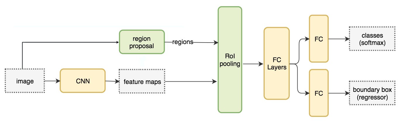
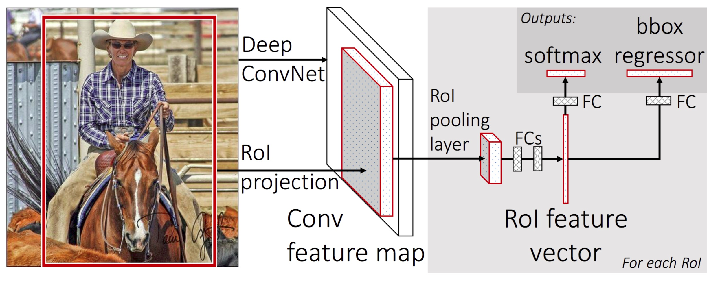
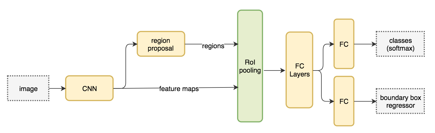
Fast R-CNN ²

How does Fast R-CNN work?

• Instead of extracting features for each image patch from scratch, we use a feature extractor (a CNN) to extract features for the whole image first.
• We also use an external region proposal method, like the selective search, to create ROIs which later combine with the corresponding feature maps to form patches for object detection.
• We warp the patches to a fixed size using ROI pooling and feed them to fully connected layers for classification and localization (detecting the location of the object).

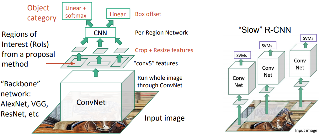
System flow:

Pseudo-code:

feature_maps = process(image)
ROIs = region_proposal(image)
for ROI in ROIs:
    patch = roi_pooling(feature_maps, ROI)
    results = detector2(patch)

• The expensive feature extraction is moving out of the for-loop. This is a significant speed improvement since it was executed for all 2000 ROIs. 👏

One major takeaway for Fast R-CNN is that the whole network (the feature extractor, the classifier, and the boundary box regressor) are trained end-to-end with multi-task losses (classification loss and localization loss). This improves accuracy.

ROI pooling

Because Fast R-CNN uses fully connected layers, we apply ROI pooling to warp the variable size ROIs into in a predefined fix size shape.

Let’s take a look at a simple example: transforming 8 × 8 feature maps into a predefined 2 × 2 shape.

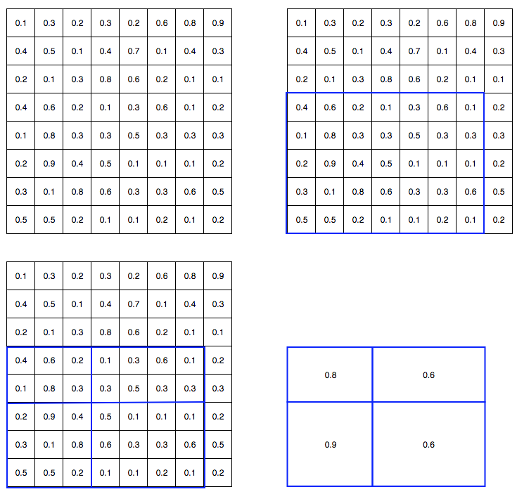
• Top left: feature maps

• Top right: we overlap the ROI (blue) with the feature maps.

• Bottom left: we split ROIs into the target dimension. For example, with our 2×2 target, we split the ROIs into 4 sections with similar or equal sizes.

• Bottom right: find the maximum for each section (i.e, max-pool within each section) and the result is our warped feature maps.

Now we get a 2 × 2 feature patch that we can feed into the classifier and box regressor.

Another gif example:

Problems of Fast R-CNN

Fast R-CNN depends on an external region proposal method like selective search. However, those algorithms run on CPU and they are slow. In testing, Fast R-CNN takes 2.3 seconds to make a prediction in which 2 seconds are for generating 2000 ROIs!!!

feature_maps = process(image)
ROIs = region_proposal(image) # Expensive!
for ROI in ROIs:
    patch = roi_pooling(feature_maps, ROI)
    results = detector2(patch)

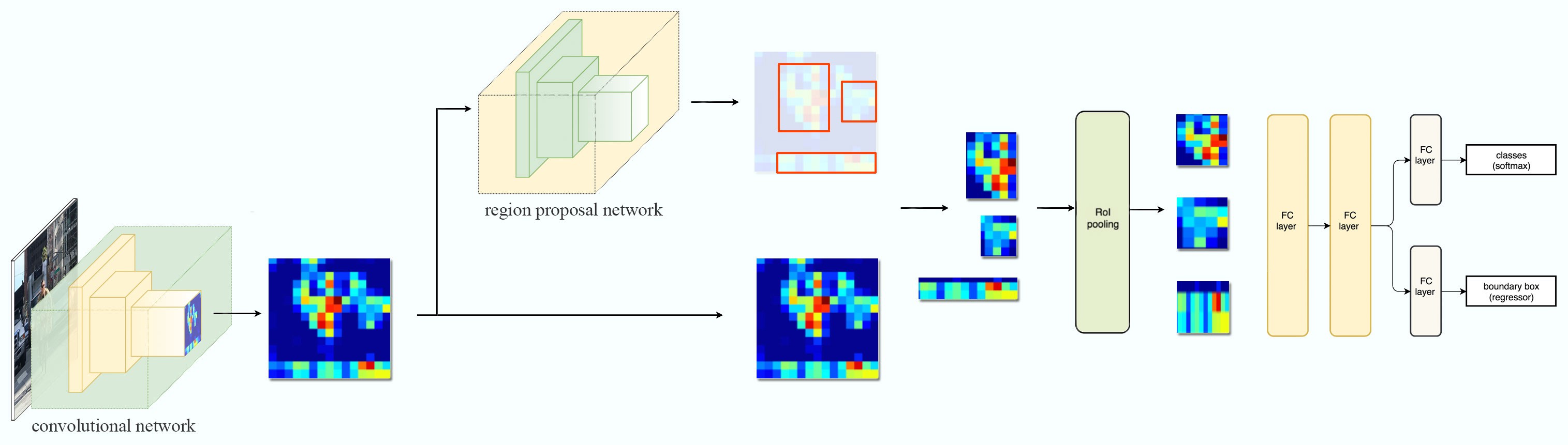
Faster R-CNN ³: Make CNN do proposals

Faster R-CNN adopts similar design as the Fast R-CNN except

• it replaces the region proposal method by an internal deep network called Region Proposal Network (RPN)
• the ROIs are derived from the feature maps instead.

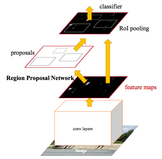
System flow: (same as Fast R-CNN)

The network flow is similar but the region proposal is now replaced by a internal convolutional network, Region Proposal Network (RPN).

Pseudo-code:

feature_maps = process(image)
ROIs = region_proposal(feature_maps) # use RPN
for ROI in ROIs:
    patch = roi_pooling(feature_maps, ROI)
    class_scores, box = detector(patch)
    class_probabilities = softmax(class_scores)

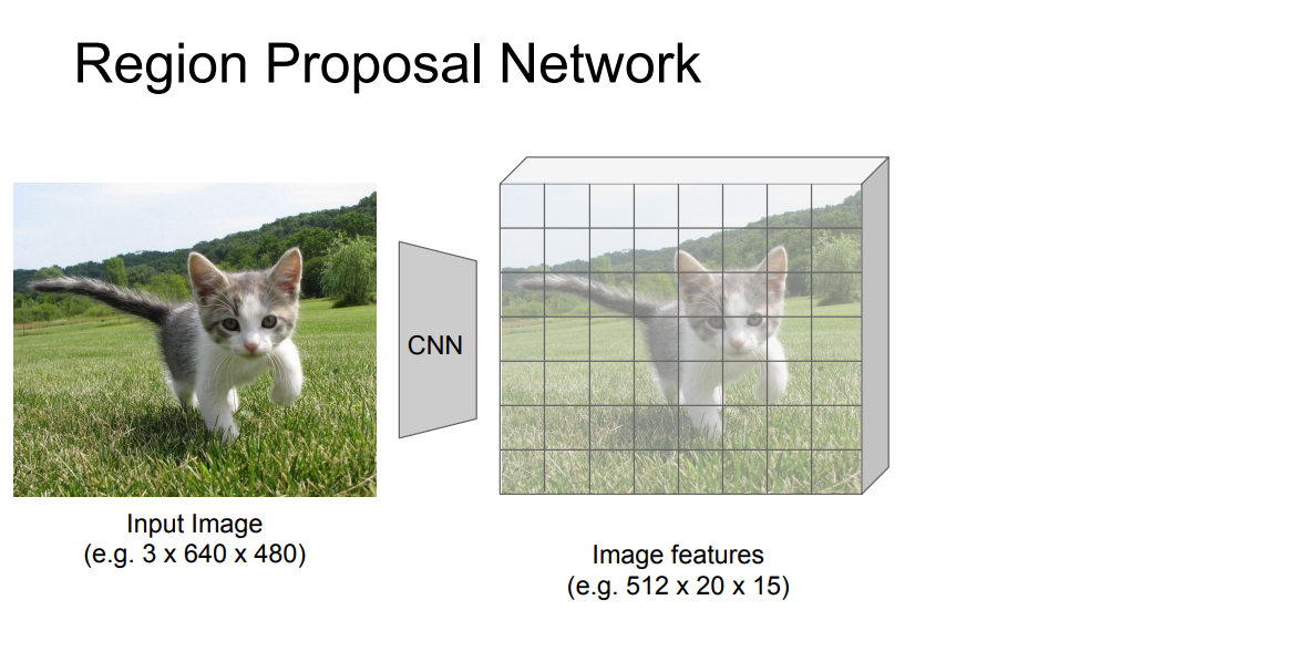
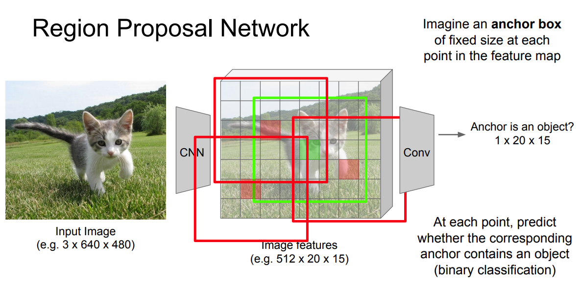
Region proposal network (RPN)

The region proposal network (RPN)

• takes the output feature maps from the first convolutional network as input

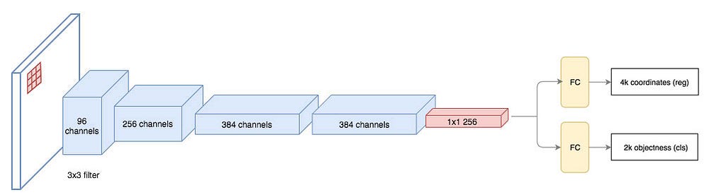
• slides 3 × 3 filters over the feature maps to make class-agnostic region proposals using a convolutional network like ZF network

  

  Other deep network likes VGG or ResNet can be used for more comprehensive feature extraction at the cost of speed.

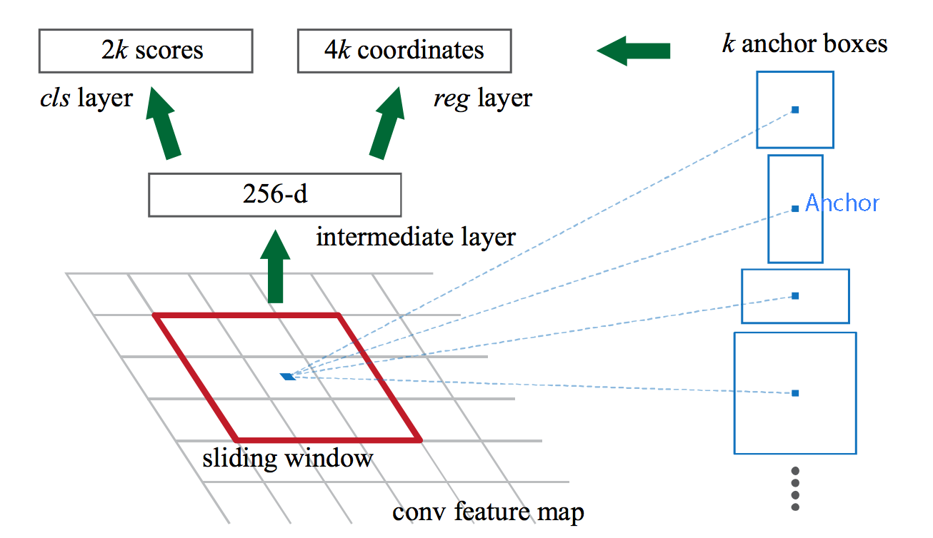
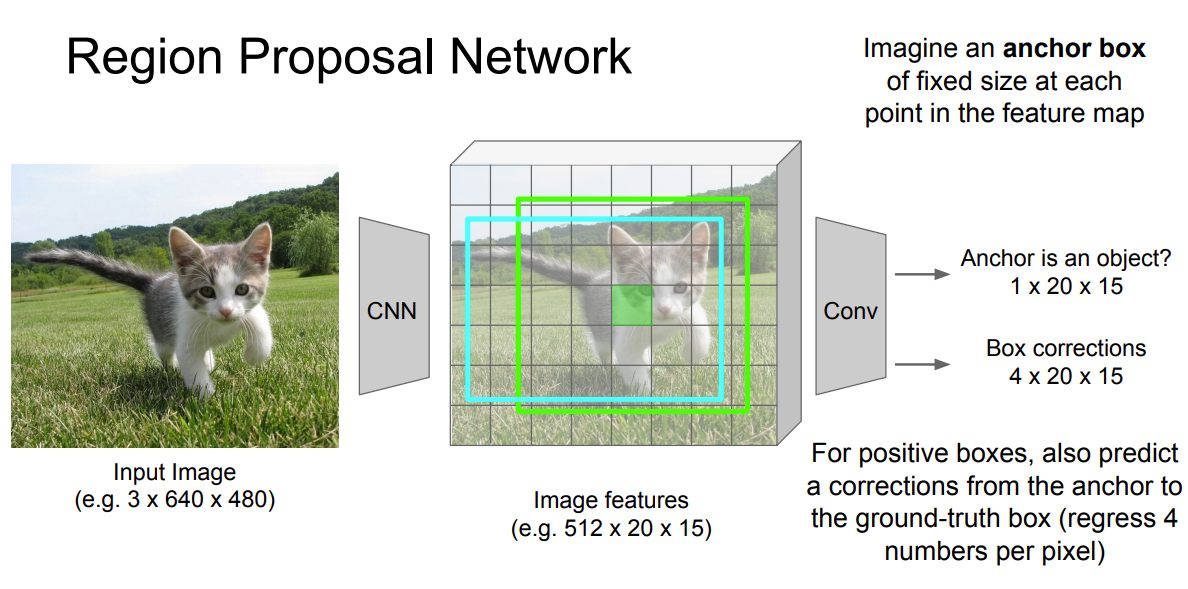
• The ZF network outputs 256 values, which is feed into 2 separate fully connected (FC) layers to predict a boundary box and 2 objectness scores.

  • The objectness measures whether the box contains an object. We can use a regressor to compute a single objectness score but for simplicity, Faster R-CNN uses a classifier with 2 possible classes: one for the “have an object” category and one without (i.e. the background class).

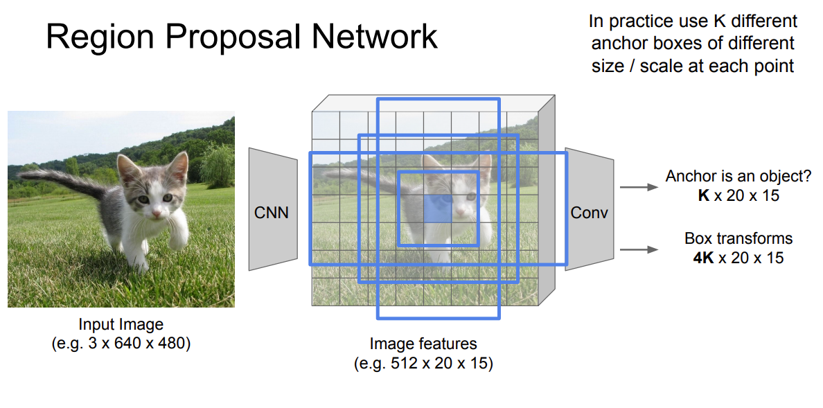
• For each location in the feature maps, RPN makes $k$ guesses

  $\Rightarrow$ RPN outputs $4 \times k$ coordinates (top-left and bottom-right $(x, y)$ coordinates) for bounding box and $2 \times k$ scores for objectness (with vs. without object) per location

  • Example: $8 \times 8$ feature maps with a $3 \times 3$ filter, and it outputs a total of $8 \times 8 \times 3$ ROIs (for $k = 3$)

    

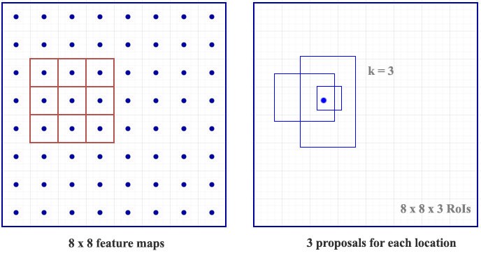
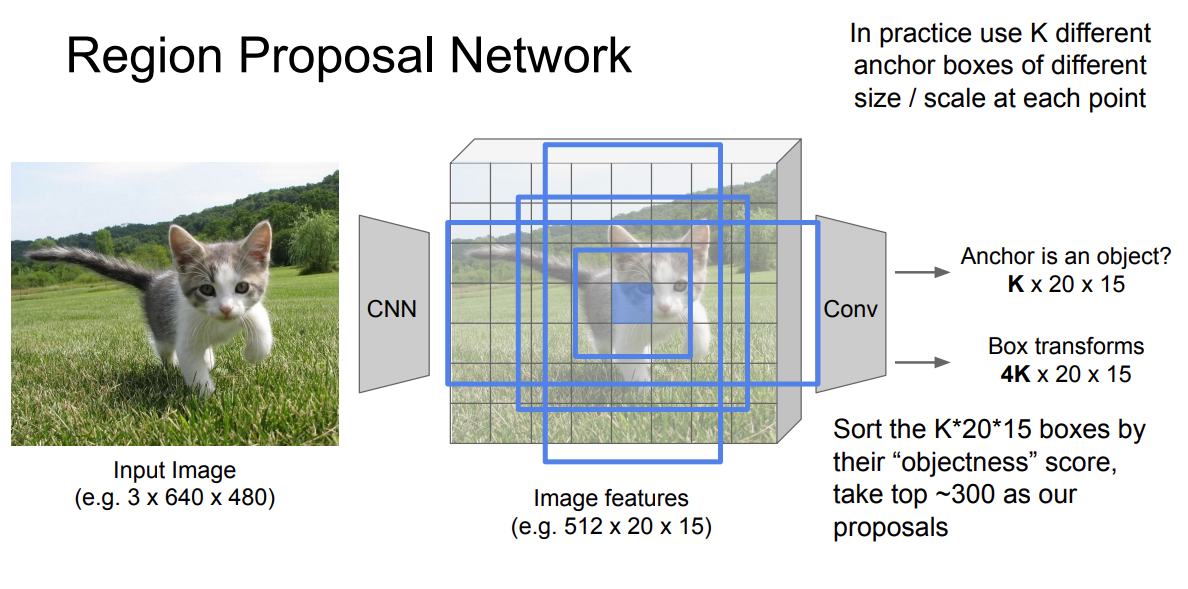
    • Here we get 3 guesses and we will refine our guesses later. Since we just need one to be correct, we will be better off if our initial guesses have different shapes and size.

      Therefore, Faster R-CNN does not make random boundary box proposals. Instead, it predicts offsets like $\delta_x, \delta_y$ that are relative to the top left corner of some reference boxes called anchors. We constraints the value of those offsets so our guesses still resemble the anchors.

      

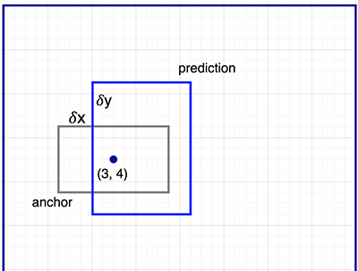
    • To make $k$ predictions per location, we need $k$ anchors centered at each location. Each prediction is associated with a specific anchor but different locations share the same anchor shapes.

      

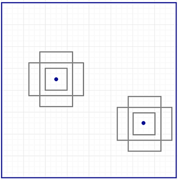
    • Those anchors are carefully pre-selected so they are diverse and cover real-life objects at different scales and aspect ratios reasonable well.

      • This guides the initial training with better guesses and allows each prediction to specialize in a certain shape. This strategy makes early training more stable and easier. 👍

• Faster R-CNN uses far more anchors. It deploys 9 anchor boxes: 3 different scales at 3 different aspect ratio. Using 9 anchors per location, it generates 2 × 9 objectness scores and 4 × 9 coordinates per location.

  

Nice example and explanation from Stanford cs231n slide

Region-based Fully Convolutional Networks (R-FCN) ⁴

💡 Idea

Let’s assume we only have a feature map detecting the right eye of a face. Can we use it to locate a face? It should. Since the right eye should be on the top-left corner of a facial picture, we can use that to locate the face.

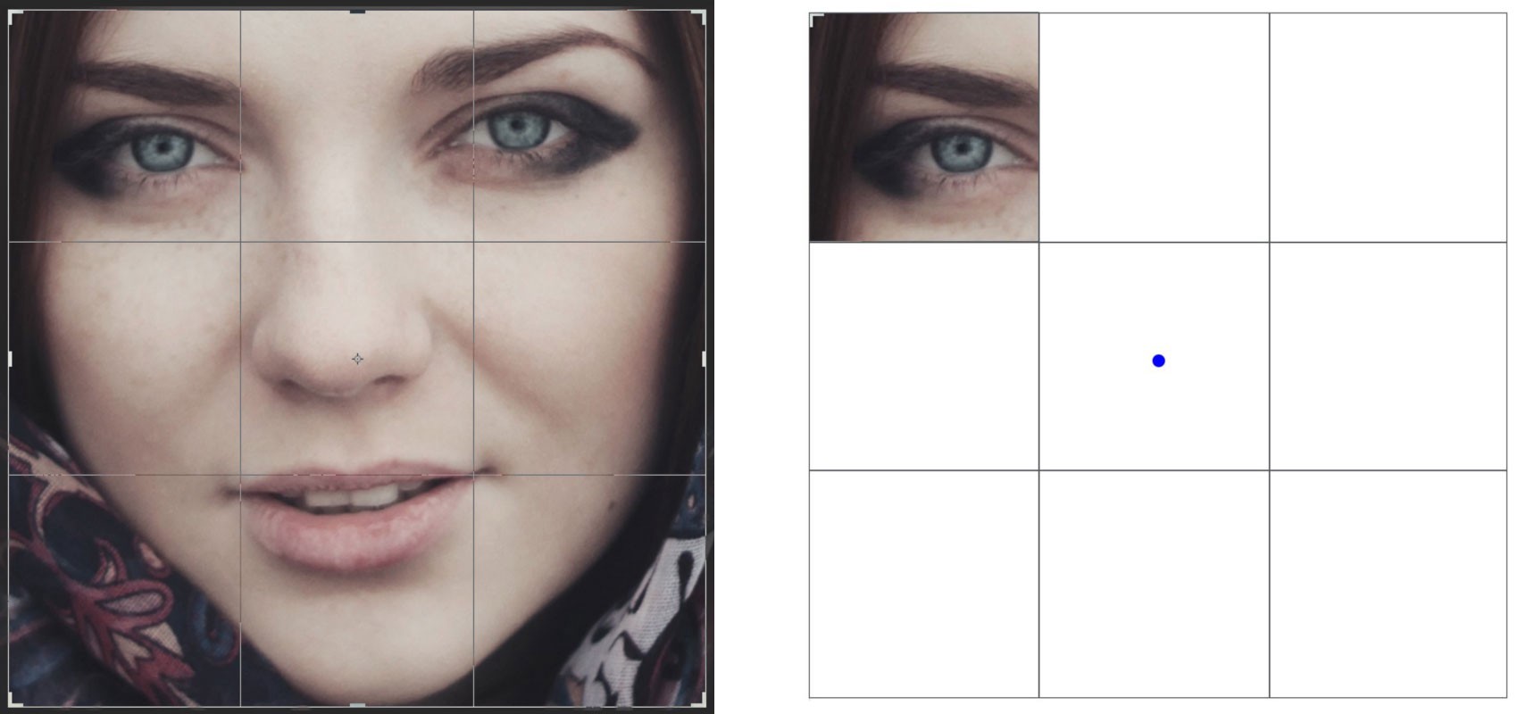
If we have other feature maps specialized in detecting the left eye, the nose or the mouth, we can combine the results together to locate the face better.

Problem of Faster R-CNN

In Faster R-CNN, the detector applies multiple fully connected layers to make predictions. With 2,000 ROIs, it can be expensive.

feature_maps = process(image)
ROIs = region_proposal(feature_maps)
for ROI in ROIs
    patch = roi_pooling(feature_maps, ROI)
    class_scores, box = detector(patch) # Expensive!
    class_probabilities = softmax(class_scores)

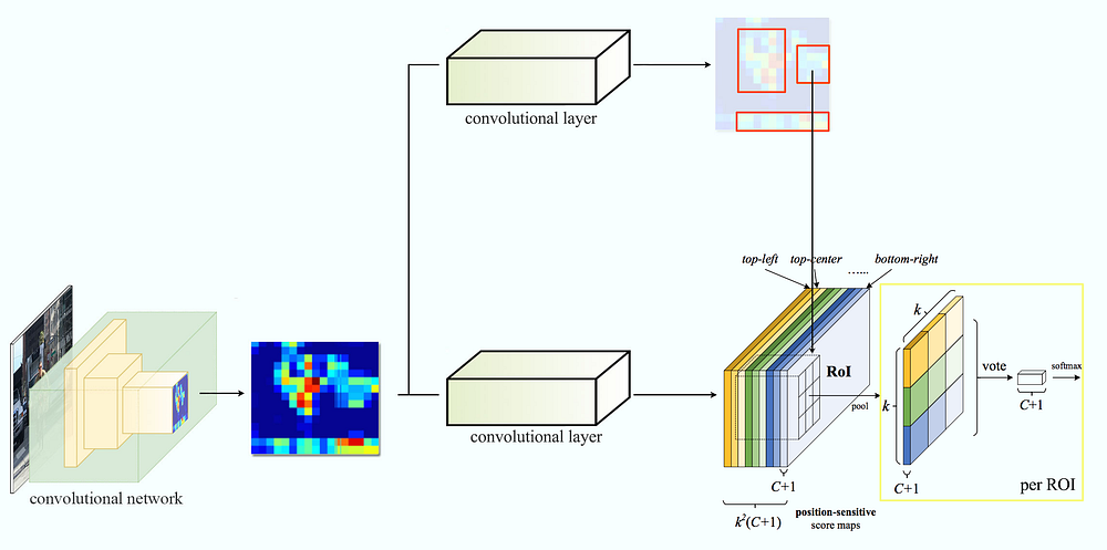
R-FCN: reduce the amount of work needed for each ROI

R-FCN improves speed by reducing the amount of work needed for each ROI. The region-based feature maps above are independent of ROIs and can be computed outside each ROI. The remaining work is then much simpler and therefore R-FCN is faster than Faster R-CNN.

Pseudo-code:

feature_maps = process(image)
ROIs = region_proposal(feature_maps)         
score_maps = compute_score_map(feature_maps)
for ROI in ROIs:
    V = region_roi_pool(score_maps, ROI)     
    class_scores, box = average(V)                   # Much simpler!
    class_probabilities = softmax(class_scores)

Position-sensitive score mapping

Let’s consider a 5 × 5 feature map M with a blue square object inside. We divide the square object equally into 3 × 3 regions.

Now, we create a new feature map from M to detect the top left (TL) corner of the square only. The new feature map looks like the one on the right below. Only the yellow grid cell [2, 2] is activated.

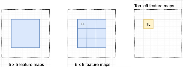
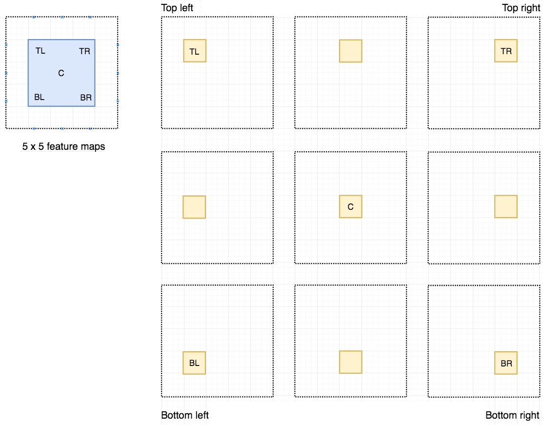
Since we divide the square into 9 parts, we can create 9 feature maps each detecting the corresponding region of the object. These feature maps are called position-sensitive score maps because each map detects (scores) a sub-region of the object.

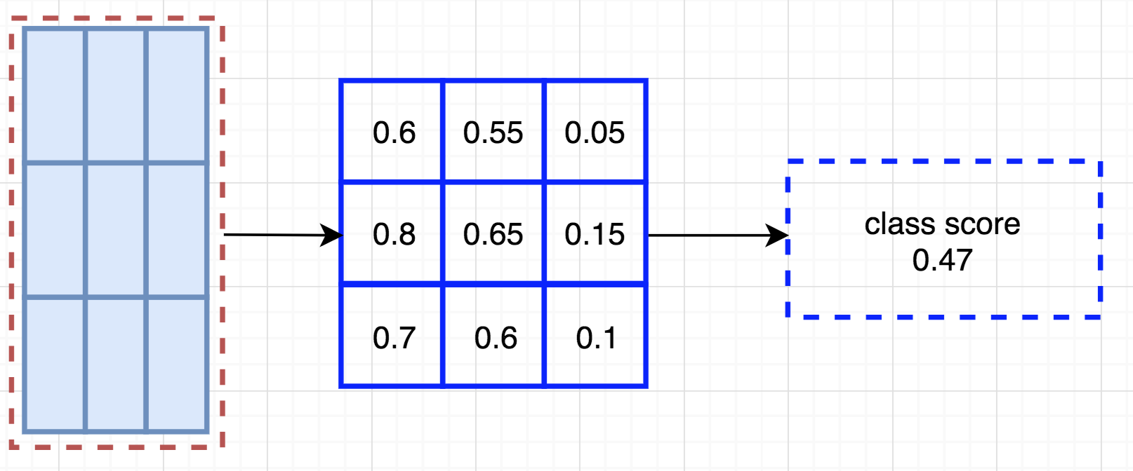
Let’s say the dotted red rectangle below is the ROI proposed. We divide it into 3 × 3 regions and ask how likely each region contains the corresponding part of the object.

For example, how likely the top-left ROI region contains the left eye. We store the results into a 3 × 3 vote array in the right diagram below. For example, vote_array[0][0] contains the score on whether we find the top-left region of the square object.

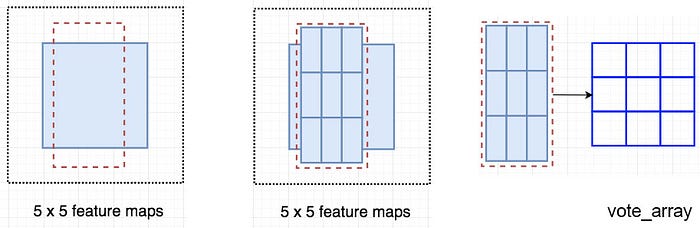
This process to map score maps and ROIs to the vote array is called position-sensitive ROI-pool.

After calculating all the values for the position-sensitive ROI pool, the class score is the average of all its elements.

Data flow

• Let’s say we have $C$ classes to detect.

• We expand it to $C + 1$ classes so we include a new class for the background (non-object). Each class will have its own $3 \times 3$ score maps and therefore a total of $(C+1) \times 3 \times 3$ score maps.

• Using its own set of score maps, we predict a class score for each class.

• Then we apply a softmax on those scores to compute the probability for each class.

Reference

• What do we learn from region based object detectors (Faster R-CNN, R-FCN, FPN)? - A nice and clear comprehensive tutorial for region-based object detectors
• Stanford CS231n slides
• 關於影像辨識，所有你應該知道的深度學習模型
• 一文读懂目标检测：R-CNN、Fast R-CNN、Faster R-CNN、YOLO、SSD
• RoI pooling: Understanding Region of Interest — (RoI Pooling)