Semantic Segmentation Overview
What is Semantic Segmentation?
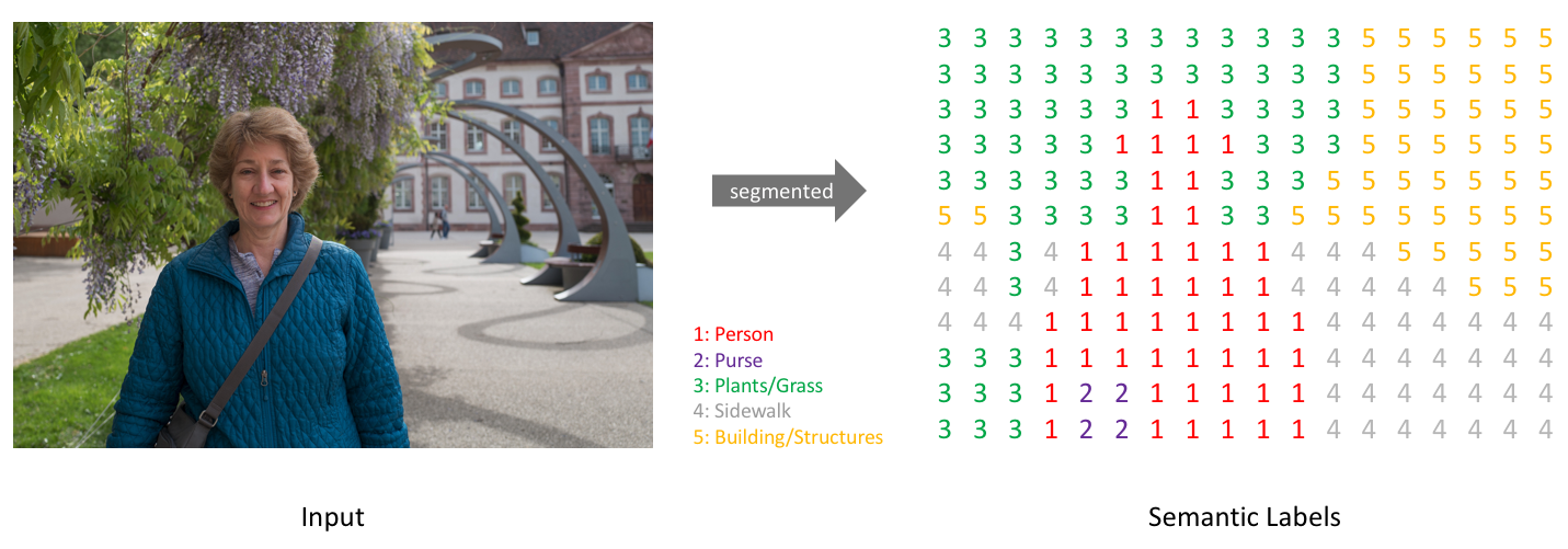
Image segmentation is a computer vision task in which we label specific regions of an image according to what’s being shown.
The goal of semantic image segmentation is to label each pixel of an image with a corresponding class of what is being represented. Because we’re predicting for every pixel in the image, this task is commonly referred to as dense prediction.
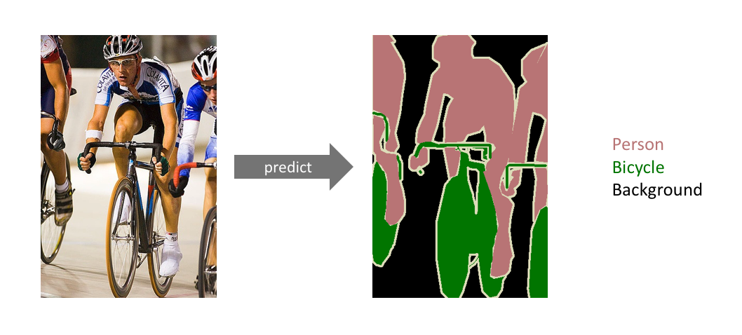
Don’t differentiate instances, only care about pixels
We’re NOT separating instances of the same class; we only care about the category of each pixel. In other words, if you have two objects of the same category in your input image, the segmentation map does not inherently distinguish these as separate objects.
Use case
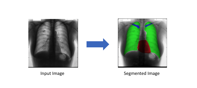
Autonomous vehicles
Medical image diagnostics
Task
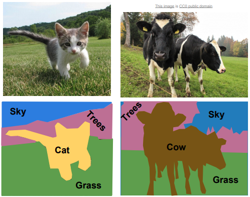
Our goal is to take either a RGB color image ($height×width×3$) or a grayscale image ($height×width×1$) and output a segmentation map where each pixel contains a class label represented as an integer ($height×width×1$).
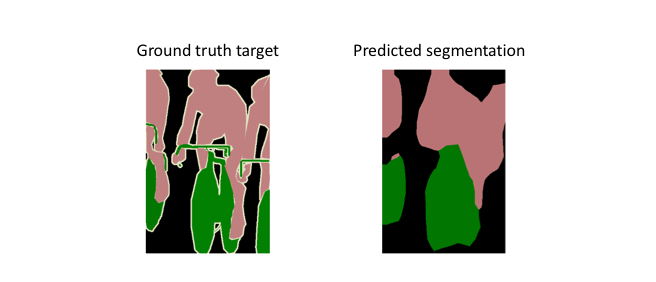
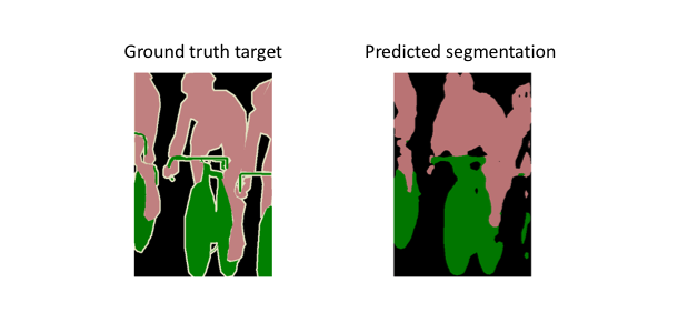
Example:
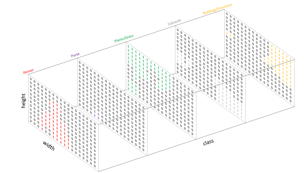
How to make prediction output?
Create our target by one-hot encoding the class labels - essentially creating an output channel for each of the possible classes.
A prediction can be collapsed into a segmentation map by taking the
argmaxof each depth-wise pixel vector.We can easily inspect a target by overlaying it onto the observation.
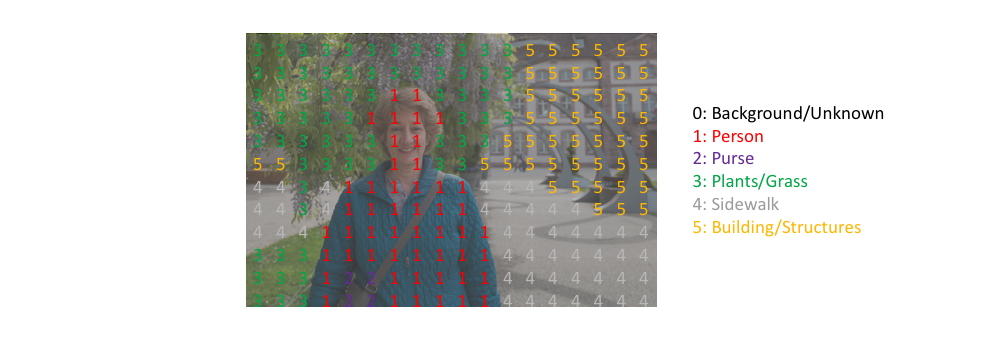
When we overlay a single channel of our target (or prediction), we refer to this as a mask which illuminates the regions of an image where a specific class is present.
Architecture
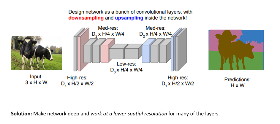
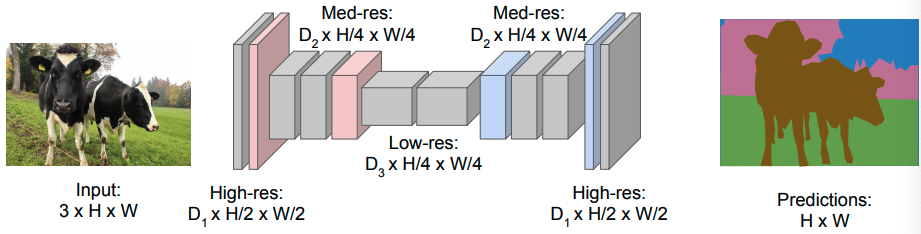
One popular approach for image segmentation models is to follow an encoder/decoder structure
- We downsample the spatial resolution of the input, developing lower-resolution feature mappings which are learned to be highly efficient at discriminating between classes
- then upsample the feature representations into a full-resolution segmentation map.
Methods for upsampling
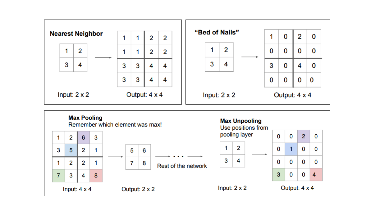
Unpooling operations
Whereas pooling operations downsample the resolution by summarizing a local area with a single value (ie. average or max pooling), “unpooling” operations upsample the resolution by distributing a single value into a higher resolution.
Transpose convolutions
Transpose convolutions are by far the most popular approach as they allow for us to develop a learned upsampling.
Typical convolution operation
- take the dot product of the values currently in the filter’s view
- produce a single value for the corresponding output position.
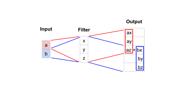
A transpose convolution essentially does the opposite
take a single value from the low-resolution feature map
multiply all of the weights in our filter by this value, projecting those weighted values into the output feature map.
For filter sizes which produce an overlap in the output feature map (eg. 3x3 filter with stride 2), the overlapping values are simply added together.
(Unfortunately, this tends to produce a checkerboard artifact in the output and is undesirable, so it’s best to ensure that your filter size does not produce an overlap.)
Fully convolutional networks
The approach of using a “fully convolutional” network trained end-to-end, pixels-to-pixels for the task of image segmentation was introduced by Long et al. in late 2014.
adapting existing, well-studied image classification networks (eg. AlexNet) to serve as the encoder module of the network
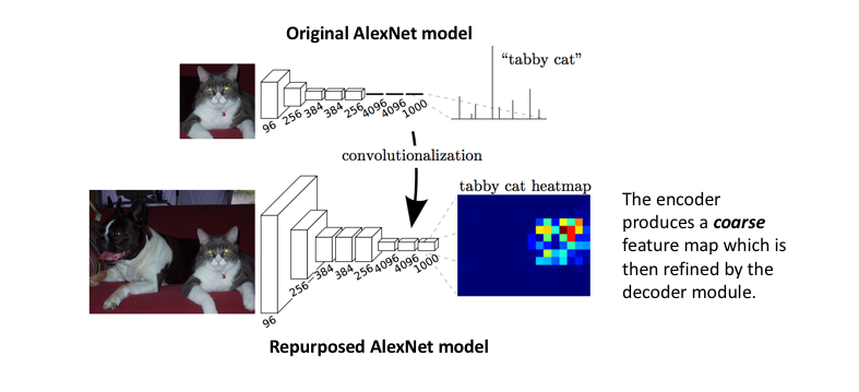
appending a decoder module with transpose convolutional layers to upsample the coarse feature maps into a full-resolution segmentation map.
However, because the encoder module reduces the resolution of the input by a factor of 32, the decoder module struggles to produce fine-grained segmentations 🤪
Adding skip connections
The authors address this tension by slowly upsampling (in stages) the encoded representation, adding “skip connections” from earlier layers, and summing these two feature maps. These skip connections from earlier layers in the network (prior to a downsampling operation) should provide the necessary detail in order to reconstruct accurate shapes for segmentation boundaries.
Indeed, we can recover more fine-grain detail with the addition of these skip connections.
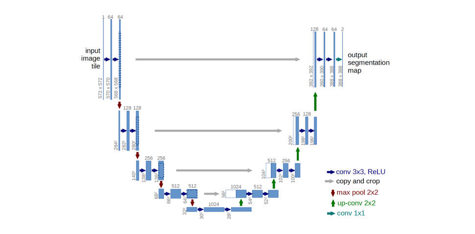
U-net
Ronneberger et al. improve upon the “fully convolutional” architecture primarily through expanding the capacity of the decoder module of the network.
They propose the U-Net architecture which “consists of a contracting path to capture context and a symmetric expanding path that enables precise localization.” This simpler architecture has grown to be very popular and has been adapted for a variety of segmentation problems.
Metrics
Intuitively, a successful prediction is one which maximizes the overlap between the predicted and true objects. Two related but different metrics for this goal are the Dice and Jaccard coefficients (or indices): $$ Dice(A, B) = \frac{2 |A \cap B|}{|A|+|B|}, \qquad Jaccard(A, B) = \frac{|A \cap B|}{|A \cup B|} $$
- $A, B$: two segmentation masks for a given class (but the formulas are general, that is, you could calculate this for anything, e.g. a circle and a square)
- $|\cdot|$: norm (for images, the area in pixels)
- $\cap, \cup$: intersection and union operators.
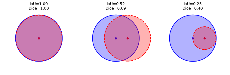
Both the Dice and Jaccard indices are bounded between 0 (when there is no overlap) and 1 (when A and B match perfectly). The Jaccard index is also known as Intersection over Union (IoU).
Here is an illustration of the Dice and IoU metrics given two circles representing the ground truth and the predicted masks for an arbitrary object class:
In terms of the confusion matrix, the metrics can be rephrased in terms of true/false positives/negatives: $$ Dice = \frac{2 TP}{2TP+FP+FN}, \qquad Jaccard = IoU = \frac{TP}{TP+FP+FN} $$
Intersection over Union (IoU)
The Intersection over Union (IoU) metric, also referred to as the Jaccard index, is essentially a method to quantify the percent overlap between the target mask and our prediction output.
Quite simply, the IoU metric measures the number of pixels common between the target and prediction masks divided by the total number of pixels present across both masks. $$ IoU = \frac{{target \cap prediction}}{{target \cup prediction}} $$ The IoU score is calculated for each class separately and then averaged over all classes to provide a global, mean IoU score of our semantic segmentation prediction.
Numpy implementation
intersection = np.logical_and(target, prediction)
union = np.logical_or(target, prediction)
iou_score = np.sum(intersection) / np.sum(union)
Example
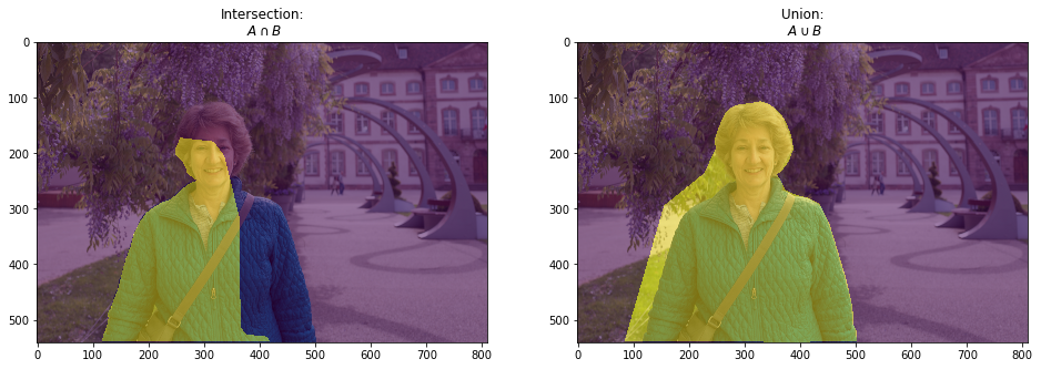
Let’s say we’re tasked with calculating the IoU score of the following prediction, given the ground truth labeled mask.
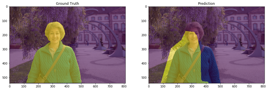
The intersection ($A∩B$) is comprised of the pixels found in both the prediction mask and the ground truth mask, whereas the union ($A∪B$) is simply comprised of all pixels found in either the prediction or target mask.
Pixel accuracy
Simply report the percent of pixels in the image which were correctly classified. The pixel accuracy is commonly reported for each class separately as well as globally across all classes.
When considering the per-class pixel accuracy we’re essentially evaluating a binary mask: $$ accuracy = \frac{{TP + TN}}{{TP + TN + FP + FN}} $$ However, this metric can sometimes provide misleading results when the class representation is small within the image, as the measure will be biased in mainly reporting how well you identify negative case (ie. where the class is not present).
Loss function
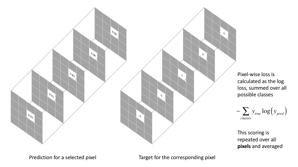
Pixel-wise cross entropy loss
This loss examines each pixel individually, comparing the class predictions (depth-wise pixel vector) to our one-hot encoded target vector.
However, because the cross entropy loss evaluates the class predictions for each pixel vector individually and then averages over all pixels, we’re essentially asserting equal learning to each pixel in the image. This can be a problem if your various classes have unbalanced representation in the image, as training can be dominated by the most prevalent class.
Dice loss
Another popular loss function for image segmentation tasks is based on the Dice coefficient, which is essentially a measure of overlap between two samples.
This measure ranges from 0 to 1 where a Dice coefficient of 1 denotes perfect and complete overlap. The Dice coefficient was originally developed for binary data, and can be calculated as: $$ Dice = \frac{{2\left| {A \cap B} \right|}}{{\left| A \right| + \left| B \right|}} $$
- ${\left| {A \cap B} \right|}$: common elements between sets $A$ and $B$
- $|A|$: number of elements in set $A$ (and likewise for set $B$).
To evaluate a Dice coefficient on predicted segmentation masks, we can approximate $|A ∩ B|$ as the element-wise multiplication between the prediction and target mask, and then sum the resulting matrix:

Because our target mask is binary, we effectively zero-out any pixels from our prediction which are not “activated” in the target mask. For the remaining pixels, we are essentially penalizing low-confidence predictions; a higher value for this expression, which is in the numerator, leads to a better Dice coefficient.
In order to formulate a loss function which can be minimized, we’ll simply use $$ 1 - Dice $$ This loss function is known as the soft Dice loss because we directly use the predicted probabilities instead of thresholding and converting them into a binary mask.
With respect to the neural network output, the numerator is concerned with the common activations between our prediction and target mask, where as the denominator is concerned with the quantity of activations in each mask separately. This has the effect of normalizing our loss according to the size of the target mask such that the soft Dice loss does not struggle learning from classes with lesser spatial representation in an image.
Reference
🔥 Overview: An overview of semantic image segmentation.
Segmentation metrics: