👍 CNN Intuition and Visualization
Intuition
A CNN model can be thought as a combination of two components:
feature extraction part
The convolution + pooling layers perform feature extraction. For example given an image, the convolution layer detects features such as two eyes, long ears, four legs, a short tail and so on.
classification part
The fully connected layers then act as a classifier on top of these features, and assign a probability for the input image being a dog.
The convolution layers are the main powerhouse of a CNN model. Automatically detecting meaningful features given only an image and a label is not an easy task. The convolution layers learn such complex features by building on top of each other. The first layers detect edges, the next layers combine them to detect shapes, to following layers merge this information to infer that this is a nose. To be clear, the CNN doesn’t know what a nose is. By seeing a lot of them in images, it learns to detect that as a feature. The fully connected layers learn how to use these features produced by convolutions in order to correctly classify the images.
Visualization
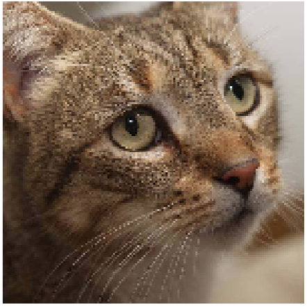
Let’s say this is our originial input image:
And we will use VGG as our CNN architectures.
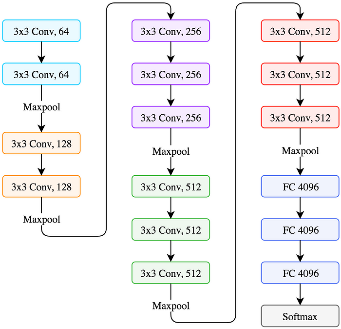
We will visualize 3 components of the VGG model:
- Feature maps
- Convnet filters
- Class output
Feature Maps Visualization
Recap of CONV-layer:
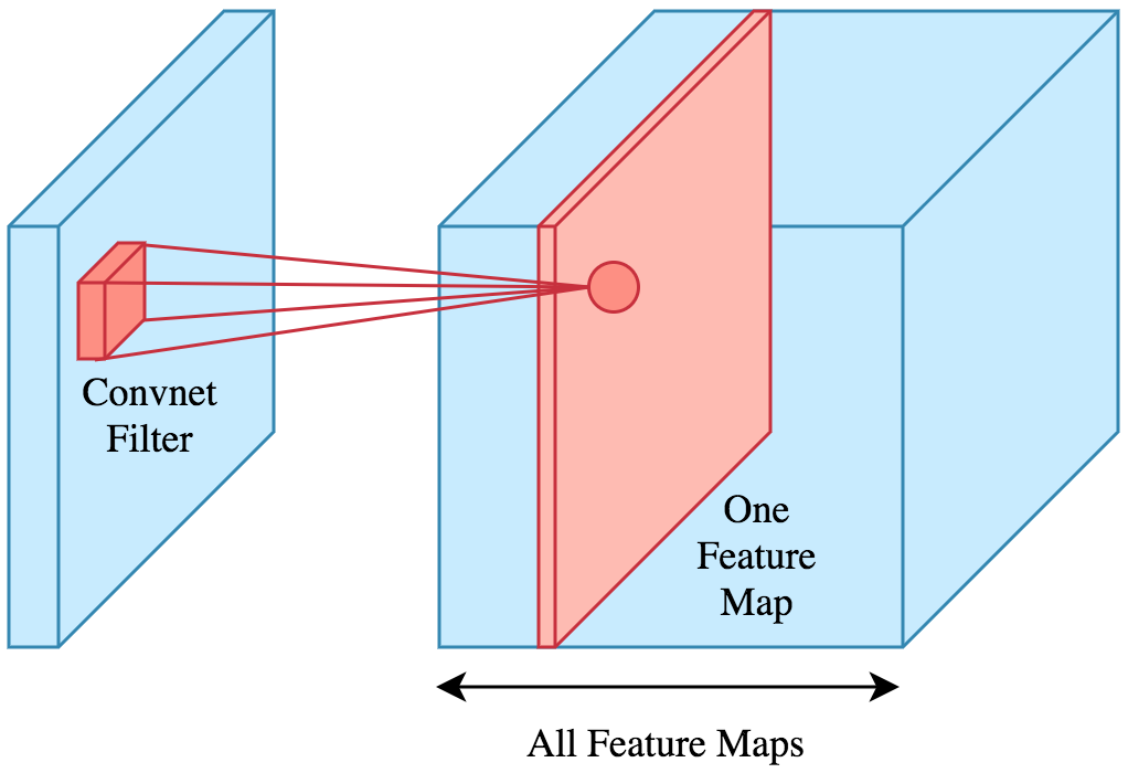
- Filter operates on the input performing the convolution operation and as a result we get a feature map.
- We use multiple filters and stack the resulting feature maps together to obtain an output volume.
We will visualize the feature maps to see how the input is transformed passing through the convolution layers. The feature maps are also called intermediate activations since the output of a layer is called the activation.
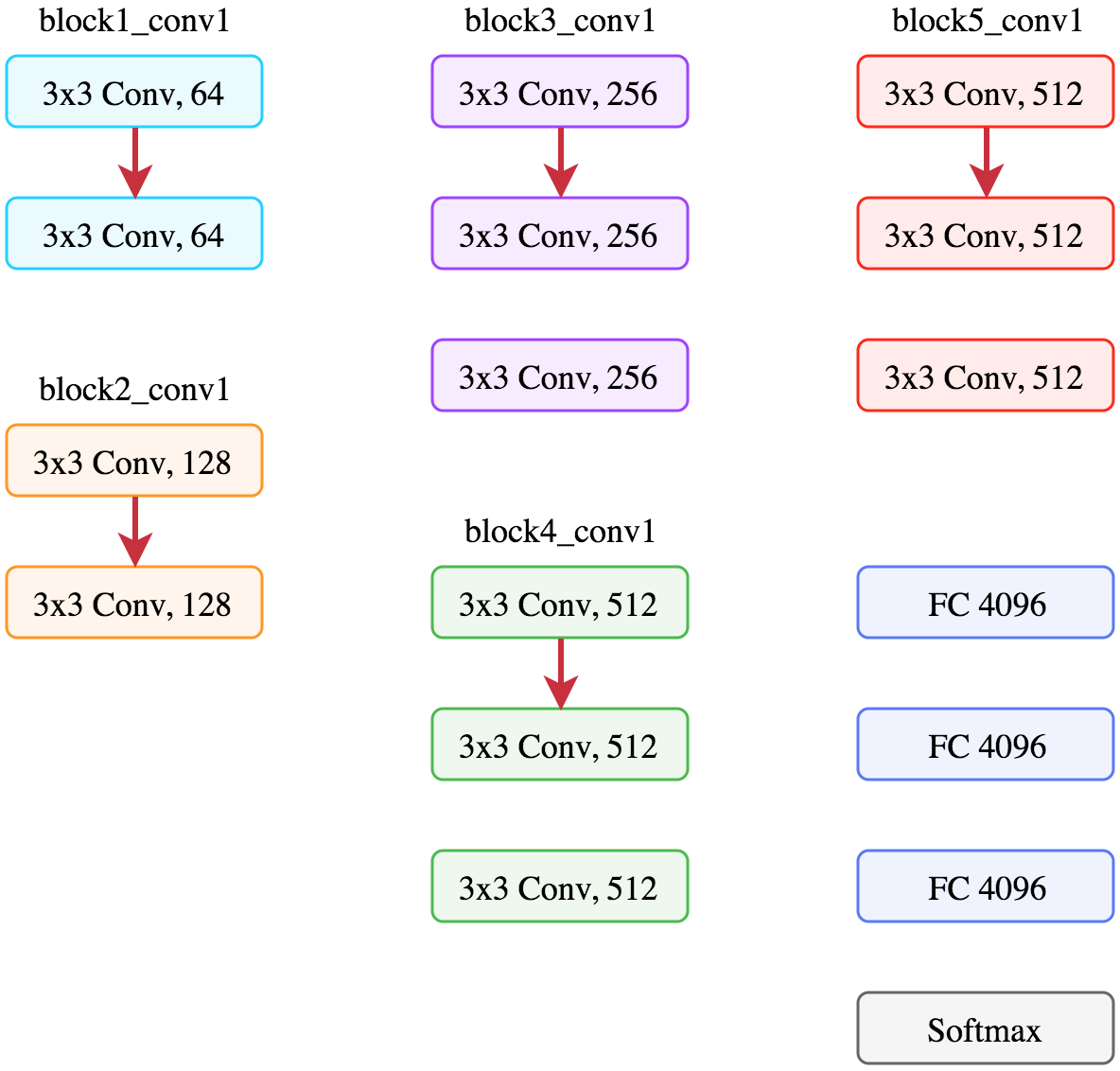
blockX_convY. For example the second filter in the third convolution block is called block3_conv2.Now let’s visualize the feature maps corresponding to the first convolution of each block, the red arrows in the figure below.
The following figure displays the first 8 feature maps per layer. Notice that there’re more than 8 feature maps per layer.
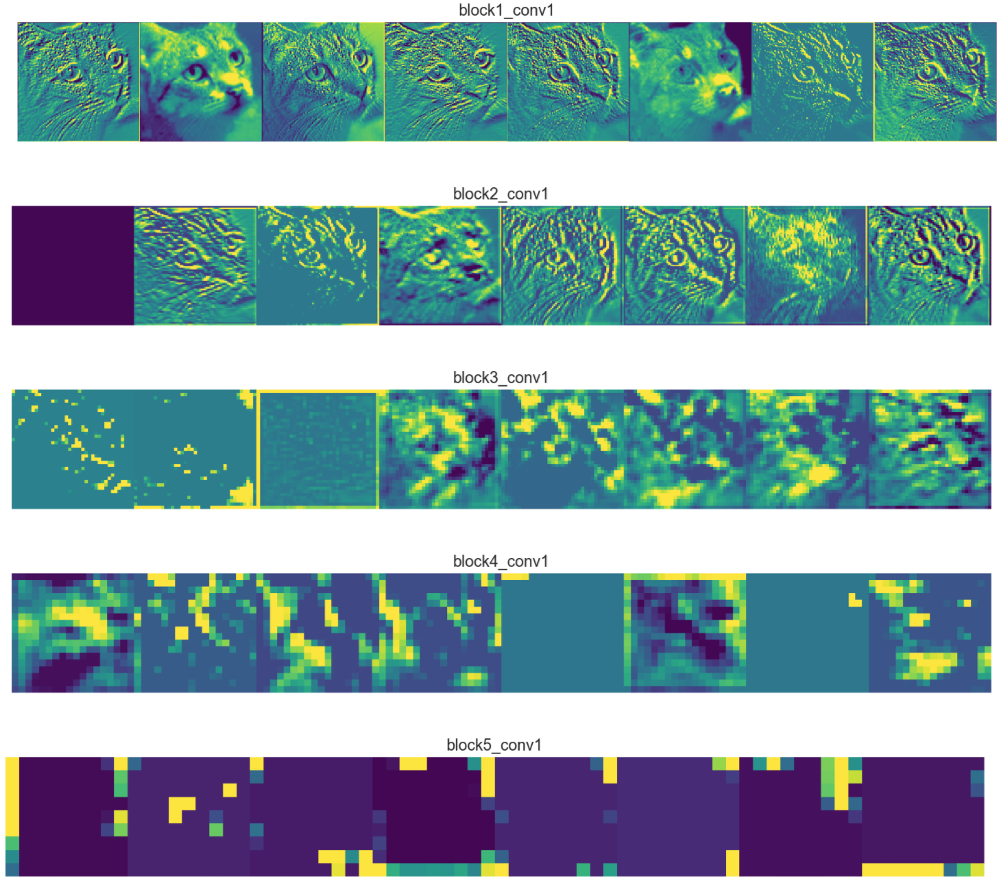
Looking at one feature map per layer, we can obtain some interesting observations:
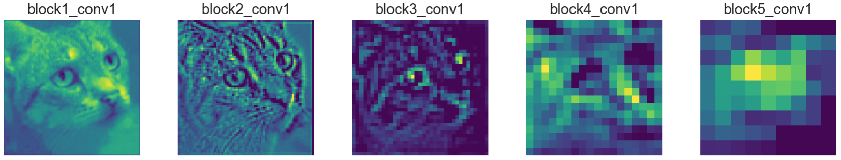
The first layer feature maps (
block1_conv1) retain most of the information present in the image. In CNN architectures the first layers usually act as edge detectors.As we go deeper into the network, the feature maps look less like the original image and more like an abstract representation of it.
- In
block3_conv1the cat is somewhat visible, but after that it becomes unrecognizable. - The reason is that deeper feature maps encode high level concepts like “cat nose” or “dog ear” while lower level feature maps detect simple edges and shapes. That’s why deeper feature maps contain less information about the image and more about the class of the image. They still encode useful features, but they are less visually interpretable by us.
- The feature maps become sparser as we go deeper, meaning the filters detect less features.
- It makes sense because the filters in the first layers detect simple shapes, and every image contains those.
- But as we go deeper we start looking for more complex stuff like “dog tail” and they don’t appear in every image. That’s why in the first figure with 8 filters per layer, we see more of the feature maps as blank as we go deeper (
block4_conv1andblock5_conv1).
- In
CONV Filters and Class Output Visualization
Check out this great article: Applied Deep Learning - Part 4: Convolutional Neural Networks
Interactive CNN Visualization
For real-time, dynamic, and interactive CNN visualization, I highly recommend CNN Explainer.