Multilayer Perceptron and Backpropagation
Multi-Layer Perceptron (MLP)
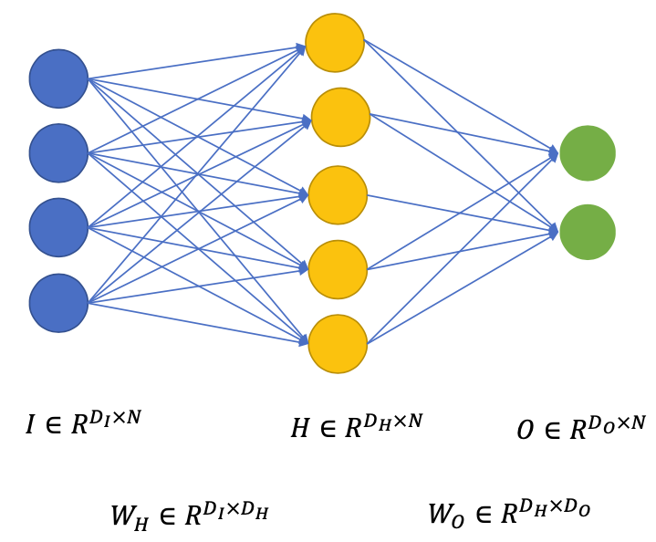
Input layer $I \in R^{D_{I} \times N}$
How we initially represent the features
Mini-batch processing with $N$ inputs
Weight matrices
Input to Hidden: $W_{H} \in R^{D_{I} \times D_{H}}$
Hidden to Output: $W_{O} \in R^{D_{H} \times D_{O}}$
Hidden layer(s) $H \in R^{D_{H} \times N}$ $$ H = W_{H}I + b_H $$
$$ \widehat{H}_j = f(H_j) $$
- $f$: non-linear activation function
Output layer $O \in R^{D_{O} \times N}$
- The value of the target function that the network approximates $$ O = W_O \widehat{H} + b_O $$
Backpropagation
Loss function $$ L = \frac{1}{2}(O - Y)^2 $$
Achieve minimum $L$: Stochastic Gradient Descent
Calculate $\frac{\delta L}{\delta w}$ for each parameter $w$
Update the parameters $$ w:=w-\alpha \frac{\delta L}{\delta w} $$
Compute the gradients: Backpropagation (Backprop)
- Output layer
$$ \begin{aligned} \frac{\delta L}{\delta O} &=(O-Y) \\ \\ \frac{\delta L}{\delta \widehat{H}} &=W_{O}^{T} \color{red}{\frac{\delta L}{\delta O}} \\ \\ \frac{\delta L}{\delta W_{O}} &= {\color{red}{\frac{\delta L}{\delta O} }}\widehat{H}^{T} \\ \\ \frac{\delta L}{\delta b_{O}} &= \color{red}{\frac{\delta L}{\delta O}} \end{aligned} $$
(Red: terms previously computed)
Hidden layer (assuming $\widehat{H}=\operatorname{sigmoid}(H)$ ) $$ \frac{\delta L}{\delta H}={\color{red}{\frac{\delta L}{\delta \hat{H}}}} \odot \widehat{H} \odot(1-\widehat{H}) $$ ($\odot$: element-wise multiplication)
Input layer
$$ \begin{array}{l} \frac{\delta L}{\delta W_{H}}={\color{red}{\frac{\delta L}{\delta H}}} I^{T} \\ \\ \frac{\delta L}{\delta b_{H}}={\color{red}{\frac{\delta L}{\delta H}}} \end{array} $$
Gradients for vectorized operations
When dealing with matrix and vector operations, we must pay closer attention to dimensions and transpose operations.
Matrix-Matrix multiply gradient. Possibly the most tricky operation is the matrix-matrix multiplication (which generalizes all matrix-vector and vector-vector) multiply operations:
(Example from cs231n)
# forward pass
W = np.random.randn(5, 10)
X = np.random.randn(10, 3)
D = W.dot(X)

# now suppose we had the gradient on D from above in the circuit
dD = np.random.randn(*D.shape) # same shape as D
dW = dD.dot(X.T) #.T gives the transpose of the matrix
dX = W.T.dot(dD)
Tip: use dimension analysis!
Note that you do not need to remember the expressions for dW and dX because they are easy to re-derive based on dimensions.
For instance, we know that the gradient on the weights dW must be of the same size as W after it is computed, and that it must depend on matrix multiplication of X and dD (as is the case when both X,W are single numbers and not matrices). There is always exactly one way of achieving this so that the dimensions work out.
For example, X is of size [10 x 3] and dD of size [5 x 3], so if we want dW and W has shape [5 x 10], then the only way of achieving this is with dD.dot(X.T), as shown above.
For discussion of math details see: Not understanding derivative of a matrix-matrix product.