👍 Backpropagation Through Time (BPTT)
Recurrent neural networks (RNNs) have attracted great attention on sequential tasks. However, compared to general feedforward neural networks, it is a little bit harder to train RNNs since RNNs have feedback loops.
In this article, we dive into basics, especially the error backpropagation to compute gradients with respect to model parameters. Furthermore, we go into detail on how error backpropagation algorithm is applied on long short-term memory (LSTM) by unfolding the memory unit.
BPTT in RNN
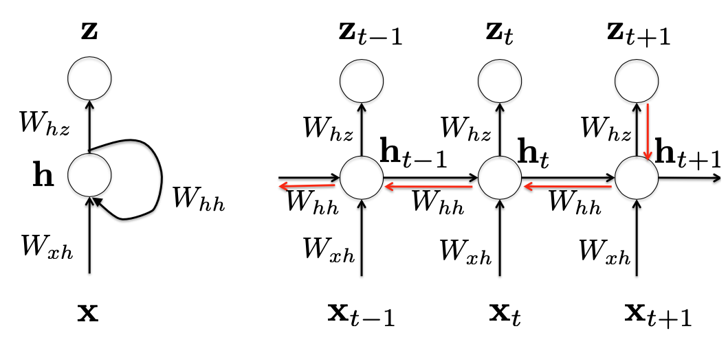
$\mathbf{x}_t$: current observation/input
$\mathbf{h}_t$: hidden state
dependent on:
- current observation $\mathbf{x}_t$
- previous hidden state $\mathbf{h}_{t-1}$
Representation: $$ \mathbf{h}_{t}=f\left(\mathbf{h}_{t-1}, \mathbf{x}_{t}\right) $$
- $f$: nonlinear mapping
$z_t$: output/prediction at time step $t$
Suppose we have the following RNN: $$ \begin{array}{l} \mathbf{h}_{t}=\tanh \left(W_{h h} \mathbf{h}_{t-1}+W_{x h} \mathbf{x}_{t}+\mathbf{b}_{\mathbf{h}}\right) \\ \alpha_t = W_{h z} \mathbf{h}_{t}+\mathbf{b}_{z}\\ z_{t}=\operatorname{softmax}\left(\alpha_t\right) \end{array} $$
Considering the varying length for each sequential data, we also assume the parameters in each time step are the same across the whole sequential analysis (Otherwise it will be hard to compute the gradients). In addition, sharing the weights for any sequential length can generalize the model well.
As for sequential labeling, we can use the maximum likelihood to estimate model parameters. In other words, we can minimize the negative log likelihood the objective function ($\to$ cross entropy) $$ \mathcal{L}(\mathbf{x}, \mathbf{y})=-\sum_{t} y_{t} \log z_{t} $$
- For simplicity, in the following we will use $\mathcal{L}$ as the objective function
- At time step $t+1$: $\mathcal{L}(t+1)=-y_{t+1}\log z_{t+1}$
Derivation
$W_{hz}$ and $b_z$
Based on the RNN above, by taking the derivative with respect to $\alpha_t$, we have (refer to derivative of softmax) $$ \frac{\partial \mathcal{L}}{\partial \alpha_{t}}=-\left(y_{t}-z_{t}\right) $$ Note the weight $W_{hz}$ is shared across all time sequence, thus we can differentiate to it at each time step and sum all together $$ \frac{\partial \mathcal{L}}{\partial W_{h z}}=\sum_{t} \frac{\partial \mathcal{L}}{\partial z_{t}} \frac{\partial z_{t}}{\partial W_{h z}} $$ Similarly, we can get the gradient w.r.t. bias $b_z$ $$ \frac{\partial \mathcal{L}}{\partial b_{z}}=\sum_{t} \frac{\partial \mathcal{L}}{\partial z_{t}} \frac{\partial z_{t}}{\partial b_{z}} $$
$W_{hh}$
Consider at time step $t \to t + 1$ in the figure above $$ \frac{\partial \mathcal{L}(t+1)}{\partial W_{h h}}=\frac{\partial \mathcal{L}(t+1)}{\partial z_{t+1}} \frac{\partial z_{t+1}}{\partial \mathbf{h}_{t+1}} \frac{\partial \mathbf{h}_{t+1}}{\partial W_{h h}} $$ Because the hidden state $\mathbf{h}_{t+1}$ partially depends on $\mathbf{h}_t$, we can use backpropagation to compute the above partial derivative. Futhermore, $W_{hh}$ is shared cross the whole time sequence. Therefore, at time step $(t-1) \to t$, we can get the partial derivative w.r.t. $W_{hh}$: $$ \frac{\partial \mathcal{L}(t+1)}{\partial W_{h h}}=\frac{\partial \mathcal{L}(t+1)}{\partial z_{t+1}} \frac{\partial z_{t+1}}{\partial \mathbf{h}_{t+1}} \frac{\partial \mathbf{h}_{t+1}}{\partial \mathbf{h}_{t}} \frac{\partial \mathbf{h}_{t}}{\partial W_{h h}} $$ Thus, at the time step $t + 1$, we can compute gradient w.r.t. $z_{t+1}$ and further use backpropagation through time (BPTT) from $t$ to $0$ to calculate gradient w.r.t. $W_{hh}$ (shown as the red chain in figure above). In other words, if we only consider the output $z_{t+1}$ at time step $t + 1$, we can yield the following gradient w.r.t. $W_{hh}$: $$ \frac{\partial \mathcal{L}(t+1)}{\partial W_{h h}}=\sum_{k=1}^{t+1} \frac{\partial \mathcal{L}(t+1)}{\partial z_{t+1}} \frac{\partial z_{t+1}}{\partial \mathbf{h}_{t+1}} \frac{\partial \mathbf{h}_{t+1}}{\partial \mathbf{h}_{k}} \frac{\partial \mathbf{h}_{k}}{\partial W_{h h}} $$ Example: $t = 2$
Aggregate the gradients w.r.t. $W_{hh}$ over the whole time sequence with back propagation, we can finally yield the following gradient w.r.t $W_{hh}$: $$ \frac{\partial \mathcal{L}}{\partial W_{h h}}=\sum_{t} \sum_{k=1}^{t+1} \frac{\partial \mathcal{L}(t+1)}{\partial z_{t+1}} \frac{\partial z_{t+1}}{\partial \mathbf{h}_{t+1}} \frac{\partial \mathbf{h}_{t+1}}{\partial \mathbf{h}_{k}} \frac{\partial \mathbf{h}_{k}}{\partial W_{h h}} $$
$W_{xh}$
Similar to $W_{hh}$, we consider the time step $t + 1$ (only contribution from $\mathbf{x}_{t+1}$) and calculate the gradient w.r.t. $W_{xh}$: $$ \frac{\partial \mathcal{L}(t+1)}{\partial W_{x h}}=\frac{\partial \mathcal{L}(t+1)}{\partial \mathbf{h}_{t+1}} \frac{\partial \mathbf{h}_{t+1}}{\partial W_{x h}} $$ Because $\mathbf{h}_{t}$ and $\mathbf{x}_t$ both make contribution to $\mathbf{h}_{t+1}$, we need to back propagate to $\mathbf{h}_{t}$ as well. If we consider the contribution from the time step $t$, we can further get $$ \begin{aligned} & \frac{\partial \mathcal{L}(t+1)}{\partial W_{x h}}=\frac{\partial \mathcal{L}(t+1)}{\partial \mathbf{h}_{t+1}} \frac{\partial \mathbf{h}_{t+1}}{\partial W_{x h}}+\frac{\partial \mathcal{L}(t+1)}{\partial \mathbf{h}_{t}} \frac{\partial \mathbf{h}_{t}}{\partial W_{x h}} \\ =& \frac{\partial \mathcal{L}(t+1)}{\partial \mathbf{h}_{t+1}} \frac{\partial \mathbf{h}_{t+1}}{\partial W_{x h}}+\frac{\partial \mathcal{L}(t+1)}{\partial \mathbf{h}_{t+1}} \frac{\partial \mathbf{h}_{t+1}}{\partial \mathbf{h}_{t}} \frac{\partial \mathbf{h}_{t}}{\partial W_{x h}} \end{aligned} $$ Thus, summing up all contributions from $t$ to $0$ via backpropagation, we can yield the gradient at the time step $t + 1$: $$ \frac{\partial \mathcal{L}(t+1)}{\partial W_{x h}}=\sum_{k=1}^{t+1} \frac{\partial \mathcal{L}(t+1)}{\partial \mathbf{h}_{t+1}} \frac{\partial \mathbf{h}_{t+1}}{\partial \mathbf{h}_{k}} \frac{\partial \mathbf{h}_{k}}{\partial W_{x h}} $$ Example: $t=2$
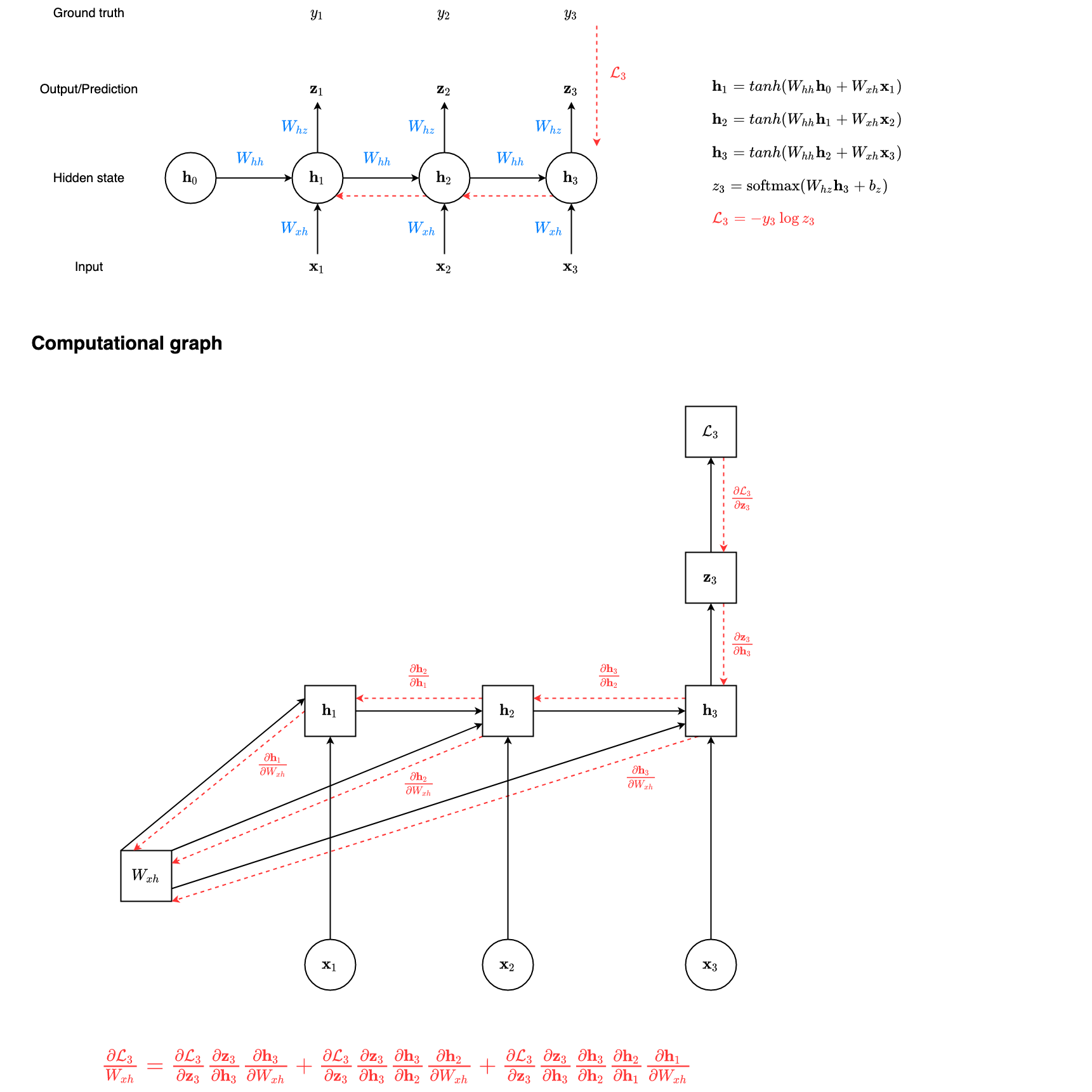
Further, we can take derivative w.r.t. $W_{xh}$ over the whole sequence as $$ \frac{\partial \mathcal{L}}{\partial W_{x h}}=\sum_{t} \sum_{k=1}^{t+1} \frac{\partial \mathcal{L}(t+1)}{\partial z_{t+1}} \frac{\partial z_{t+1}}{\partial \mathbf{h}_{t+1}} \frac{\partial \mathbf{h}_{t+1}}{\partial \mathbf{h}_{k}} \frac{\partial \mathbf{h}_{k}}{\partial W_{x h}} $$
Gradient vanishing or exploding problems
Notice that $\frac{\partial \mathbf{h}_{t+1}}{\partial \mathbf{h}_{k}}$ in the equation above indicates matrix multiplication over the sequence. And RNNs need to backpropagate gradients over a long sequence
With small values in the matrix multiplication
Gradient value will shrink layer over layer, and eventually vanish after a few time steps. Thus, the states that are far away from the current time step does not contribute to the parameters’ gradient computing (or parameters that RNNs is learning)!
$\to$ Gradient vanishing
With large values in the matrix multiplication
Gradient value will get larger layer over layer, and eventually become extremly large!
$\to$ Gradient exploding
BPTT in LSTM
The representation of LSTM here follows the one in A Gentle Tutorial of Recurrent Neural Network with Error Backpropagation.
More details about LSTM see: LSTM Summary
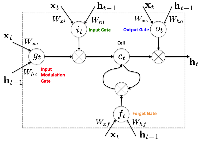
How LSTM works
Given a sequence data $\left\{\mathbf{x}_{1}, \dots,\mathbf{x}_{T}\right\}$, we have
Forget gate $$ \mathbf{f}_{t}=\sigma\left(W_{x f} \mathbf{x}_{t}+W_{h f} \mathbf{h}_{t-1}+b_{f}\right) $$
Input gate $$ \mathbf{i}_{t}=\sigma\left(W_{x i} \mathbf{x}_{t}+W_{h i} \mathbf{h}_{t-1}+b_{i}\right) $$
Candidate of new cell state $$ \mathbf{g}_{t}=\tanh \left(W_{x c} \mathbf{x}_{t}+W_{h c} \mathbf{h}_{t-1}+b_{c}\right) $$
New cell state $$ \mathbf{c}_{t}=\mathbf{f}_{t} \odot \mathbf{c}_{t-1}+\mathbf{i}_{t} \odot \mathbf{g}_{t} $$
Note
$\odot$ is a pointwise/elementwise multiplication.
$\left[\begin{array}{l} x_{1} \\ x_{2} \end{array}\right] \odot\left[\begin{array}{l} y_{1} \\ y_{2} \end{array}\right]=\left[\begin{array}{l} x_{1} y_1 \\ x_{2} y_{2} \end{array}\right]$
Output gate $$ \mathbf{o}_{t}=\sigma\left(W_{x o} \mathbf{x}_{t}+W_{h o} \mathbf{h}_{t-1}+b_{o}\right) $$
New hidden state (and output) $$ \mathbf{h}_{t}=\mathbf{o}_{t} \odot \tanh \left(\mathbf{c}_{t}\right), \quad z_{t}=\operatorname{softmax}\left(W_{h z} \mathbf{h}_{t}+b_{z}\right) $$
Derivatives
At the time step $t$:
- $\mathbf{h}_{t}=\mathbf{o}_{t} \circ \tanh \left(\mathbf{c}_{t}\right)\Rightarrow $
- $d \mathbf{o}_{t}=\tanh \left(\mathbf{c}_{t}\right) d \mathbf{h}_{t}$
- $d \mathbf{c}_{t}=\left(1-\tanh \left(\mathbf{c}_{t}\right)^{2}\right) \mathbf{o}_{t} d \mathbf{h}_{t}$ (see: Derivation of $tanh$)
- $\mathbf{c}_{t}=\mathbf{f}_{t} \circ \mathbf{c}_{t-1}+\mathbf{i}_{t} \circ \mathbf{g}_{t} \Rightarrow$
- $d \mathbf{i}_{t}=\mathbf{g}_{t} d \mathbf{c}_{t}$
- $d \mathbf{g}_{t}=\mathbf{i}_{t} d \mathbf{c}_{t}$
- $d \mathbf{f}_{t}=\mathbf{c}_{t-1} d \mathbf{c}_{t}$
- $d \mathbf{c}_{t-1}+=\mathbf{f}_{t} \circ d \mathbf{c}_{t}$ (derivation see: Error propagation)
What’s more, we backpropagate activation functions over the whole sequence (As the weights $W_{xo}, W_{xi}, W_{xf}, W_{xc}$ are shared across the whole sequence, we need to take the same summation over $t$ as in RNNs): $$ \begin{aligned} d W_{x o} &=\sum_{t} \mathbf{o}_{t}\left(1-\mathbf{o}_{t}\right) \mathbf{x}_{t} d \mathbf{o}_{t} \\ d W_{x i} &=\sum_{t} \mathbf{i}_{t}\left(1-\mathbf{i}_{t}\right) \mathbf{x}_{t} d \mathbf{i}_{t} \\ d W_{x f} &=\sum_{t} \mathbf{f}_{t}\left(1-\mathbf{f}_{t}\right) \mathbf{x}_{t} d \mathbf{f}_{t} \\ d W_{x c} &=\sum\left(1-\mathbf{g}_{t}^{2}\right) \mathbf{x}_{t} d \mathbf{g}_{t} \end{aligned} $$ Similarly, we have $$ \begin{aligned} d W_{h o} &=\sum_{t} \mathbf{o}_{t}\left(1-\mathbf{o}_{t}\right) \mathbf{h}_{t-1} d \mathbf{o}_{t} \\ d W_{h i} &=\sum_{t} \mathbf{i}_{t}\left(1-\mathbf{i}_{t}\right) \mathbf{h}_{t-1} d \mathbf{i}_{t} \\ d W_{h f} &=\sum_{t} \mathbf{f}_{t}\left(1-\mathbf{f}_{t}\right) \mathbf{h}_{t-1} d \mathbf{f}_{t} \\ d W_{h c} &=\sum_{t}\left(1-\mathbf{g}_{t}^{2}\right) \mathbf{h}_{t-1} d \mathbf{g}_{t} \end{aligned} $$ Since $h_{t-1}$, hidden state at time step $t-1$, is used in forget gate, input gate, candidate of new cell state, and output gate, therefore: $$ \begin{aligned} d \mathbf{h}_{t-1} = &\mathbf{o}_{t}\left(1-\mathbf{o}_{t}\right) W_{h o} d \mathbf{o}_{t}+\mathbf{i}_{t}\left(1-\mathbf{i}_{t}\right) W_{h i} d \mathbf{i}_{t} \\ &+\mathbf{f}_{t}\left(1-\mathbf{f}_{t}\right) W_{h f} d \mathbf{f}_{t}+\left(1-\mathbf{g}_{t}^{2}\right) W_{h c} d \mathbf{g}_{t} \end{aligned} $$ Alternatively, we can derive $d \mathbf{h}_{t-1}$ from the objective function at time step $t-1$: $$ d \mathbf{h}_{t-1}=d \mathbf{h}_{t-1}+W_{h z} d z_{t-1} $$
Error backpropagation
Suppose we have the least square objective function $$ \mathcal{L}(\mathbf{x}, \theta)=\min \sum_{t} \frac{1}{2}\left(y_{t}-z_{t}\right)^{2} $$ where $\boldsymbol{\theta}=\left\{W_{h z}, W_{x o}, W_{x i}, W_{x f}, W_{x c}, W_{h o}, W_{h i}, W_{h f}, W_{h c}\right\}$ with bias ignored. For the sake of brevity, we use the following notation $$ \mathcal{L}(t)=\frac{1}{2}\left(y_{t}-z_{t}\right)^{2} $$ At time step $T$, we take derivative w.r.t. $\mathbf{c}_T$ $$ \frac{\partial \mathcal{L}(T)}{\partial \mathbf{c}_{T}}=\frac{\partial \mathcal{L}(T)}{\partial \mathbf{h}_{T}} \frac{\partial \mathbf{h}_{T}}{\partial \mathbf{c}_{T}} $$ At time step $T-1$, we take derivative of $\mathcal{L}(t-1)$ w.r.t. $\mathbf{c}_{T-1}$ as $$ \frac{\partial \mathcal{L}(T-1)}{\partial \mathbf{c}_{T-1}}=\frac{\partial \mathcal{L}(T-1)}{\partial \mathbf{h}_{T-1}} \frac{\partial \mathbf{h}_{T-1}}{\partial \mathbf{c}_{T-1}} $$
However, according to the following unfolded unit of structure,
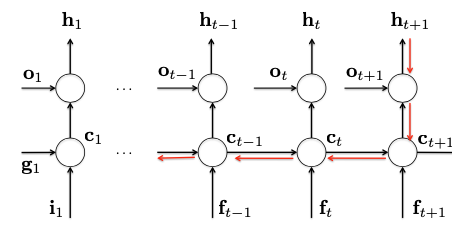
the error is not only backpropagated via $\mathcal{L}(T-1)$, but also from $\mathbf{c}_T$. Therefore, the gradient w.r.t. $\mathbf{c}_{T-1}$ should be $$ \begin{array}{ll} \frac{\partial \mathcal{L}(T-1)}{\partial \mathbf{c}_{T-1}} &= \frac{\partial \mathcal{L}(T-1)}{\partial \mathbf{c}_{T-1}}+\frac{\partial \mathcal{L}(T)}{\partial \mathbf{c}_{T-1}} \\ &=\frac{\partial \mathcal{L}(T-1)}{\partial \mathbf{h}_{T-1}} \frac{\partial \mathbf{h}_{T-1}}{\partial \mathbf{c}_{T-1}} + \underbrace{\frac{\partial \mathcal{L}(T)}{\partial \mathbf{h}_{T}} \frac{\partial \mathbf{h}_{T}}{\partial \mathbf{c}_{T}}}_{=d\mathbf{c}_T} \underbrace{\frac{\partial \mathbf{c}_{T}}{\partial \mathbf{c}_{T-1}}}_{=\mathbf{f}_T} \end{array} $$
$$ \Rightarrow \qquad d \mathbf{c}_{T-1}=d \mathbf{c}_{T-1}+\mathbf{f}_{T} \circ d \mathbf{c}_{T} $$
Parameters learning
Forward
Use the equations in How LSTM works to update states as the feedforward neural network from the time step $1$ to $T$.
Compute loss
Backward
Backpropage the error from $T$ to $1$ using equations in Derivatives. Then use gradient $d\boldsymbol{\theta}$ to update the parameters $\boldsymbol{\theta}=\left\{W_{h z}, W_{x o}, W_{x i}, W_{x f}, W_{x c}, W_{h o}, W_{h i}, W_{h f}, W_{h c}\right\}$. For example, if we use SGD, we have: $$ \boldsymbol{\theta}=\boldsymbol{\theta}-\eta d \boldsymbol{\theta} $$ where $\eta$ is the learning rate.
Derivative of softmax
$z=\operatorname{softmax}\left(W_{h z} \mathbf{h}+\mathbf{b}_{z}\right)$: predicts the probability assigned to $K$ classes.
Furthermore, we can use $1$ of $K$ (One-hot) encoding to represent the groundtruth $y$ but with probability vector to represent $z=\left[p\left(\hat{y}_{1}\right), \ldots, p\left(\hat{y}_{K}\right)\right]$. Then, we can consider the gradient in each dimension, and then generalize it to the vector case in the objective function (cross-entropy loss): $$ \mathcal{L}\left(W_{h z}, \mathbf{b}_{z}\right)=-y \log z $$ Let $$ \alpha_{j}(\Theta)=W_{h z}(:, j) \mathbf{h}_{t} $$ Then $$ p\left(\hat{y}_{j} \mid \mathbf{h}_{t} ; \Theta\right)=\frac{\exp \left(\alpha_{j}(\Theta)\right)}{\sum_{k} \exp \left(\alpha_{k}(\Theta)\right)} $$ Derivative w.r.t $\alpha_j(\Theta)$ $$ \begin{array}{ll} &\frac{\partial}{\partial \alpha_{j}} y_{j} \log p\left(\hat{y}_{j} \mid \mathbf{h}_{t} ; \Theta\right) \\ \\ =&y_{j} \left(\frac{\partial}{\partial \alpha_{j}} \log p\left(\hat{y}_{j} \mid \mathbf{h}_{t} ; \Theta\right)\right) \left(\frac{\partial}{\partial \alpha_{j}} p\left(\hat{y}_{j} \mid \mathbf{h}_{t} ; \Theta\right)\right) \\ \\ =&y_{j} \cdot \frac{1}{p\left(\hat{y}_{j} \mid \mathbf{h}_{t} ; \Theta\right)} \cdot \left(\frac{\partial}{\partial \alpha_{j}} \frac{\exp \left(\alpha_{j}(\Theta)\right)}{\sum_{k} \exp \left(\alpha_{k}(\Theta)\right)}\right) \\ \\ =&\frac{y_{j}}{p\left(\hat{y}_{j}\right)} \frac{\exp \left(\alpha_{j}(\Theta)\right) \sum_{k} \exp \left(\alpha_{k}(\Theta)\right)-\exp \left(\alpha_{j}(\Theta)\right) \exp \left(\alpha_{j}(\Theta)\right)}{\left[\sum_{k} \exp \left(\alpha_{k}(\Theta)\right)\right]^{2}} \\ \\ =& \frac{y_{j}}{p\left(\hat{y}_{j}\right)} \underbrace{\frac{\exp \left(\alpha_{j}(\Theta)\right)}{\sum_k \exp(\alpha_k(\theta))}}_{=p\left(\hat{y}_{j}\right)} \frac{\sum_k \exp(\alpha_k(\theta)) - \exp \left(\alpha_{j}(\Theta)\right)}{\sum_k \exp(\alpha_k(\theta))}\\ \\ =&y_{j} (\frac{\sum_k \exp(\alpha_k(\theta))}{\sum_k \exp(\alpha_k(\theta))} - \underbrace{\frac{\exp \left(\alpha_{j}(\Theta)\right)}{\sum_k \exp(\alpha_k(\theta))}}_{=p\left(\hat{y}_{j}\right)}) \\ \\ =&y_{j}\left(1-p\left(\hat{y}_{j}\right)\right) \end{array} $$ Similarly, $\forall k \neq j$ and its prediction $p(\hat{y}_k)$, we take the derivative w.r.t $\alpha_j(\Theta)$: $$ \begin{array}{ll} &\frac{\partial}{\partial \alpha_{j}} y_{k} \log p\left(\hat{y}_{k} \mid \mathbf{h}_{t} ; \Theta\right)\\ \\ = &\frac{y_{k}}{p\left(\hat{y}_{k}\right)} \frac{-\exp \left(\alpha_{k}(\Theta)\right) \exp \left(\alpha_{j}(\Theta)\right)}{\left[\displaystyle \sum_{s} \exp \left(\alpha_{s}(\Theta)\right)\right]^{2}} \\ \\ = &-y_{k} p\left(\hat{y}_{j}\right) \end{array} $$ We can yield the following gradient w.r.t. $\alpha_j(\Theta)$: $$ \begin{aligned} \frac{\partial p(\hat{\mathbf{y}})}{\partial \alpha_{j}} &=\sum_{j} \frac{\partial y_{j} \log p\left(\hat{y}_{j} \mid \mathbf{h}_{i} ; \Theta\right)}{\partial \alpha_{j}} \\ &=\frac{\partial \log p\left(\hat{y}_{j} \mid \mathbf{h}_{i} ; \Theta\right)}{\partial \alpha_{j}}+\sum_{k \neq j} \frac{\partial \log p\left(\hat{y}_{k} \mid \mathbf{h}_{i} ; \Theta\right)}{\partial \alpha_{j}} \\ &=\left(y_{j}-y_{j} p\left(\hat{y}_{j}\right)\right)-\left(\sum_{k \neq j} y_{k} p\left(\hat{y}_{j}\right)\right) \\ &=y_{j}-p\left(\hat{y}_{j}\right)\left(y_{j}+\sum_{k \neq j} y_{k}\right)\\ &=y_{j}-p\left(\hat{y}_{j}\right) \end{aligned} $$
$$ \begin{aligned} \Rightarrow \frac{\partial \mathcal{L}}{\partial \alpha_j} &= \frac{\partial }{\partial \alpha_j} \left(-\sum_{j} \frac{\partial y_{j} \log p\left(\hat{y}_{j} \mid \mathbf{h}_{i} ; \Theta\right)}{\partial \alpha_{j}}\right) \\ &= -\left(y_{j}-p\left(\hat{y}_{j}\right)\right) \\ &= p\left(\hat{y}_{j}\right) - y_{j} \end{aligned} $$
See also:
Derivative of tanh
$$ \begin{aligned} \frac{\partial \tanh (x)}{\partial(x)}=& \frac{\partial \frac{\sinh (x)}{\cosh (x)}}{\partial x} \\ =& \frac{\frac{\partial \sinh (x)}{\partial x} \cosh (x)-\sinh (x) \frac{\partial \cosh (x)}{\partial x}}{(\cosh (x))^{2}} \\ =& \frac{[\cosh (x)]^{2}-[\sinh (x)]^{2}}{(\cosh (x))^{2}} \\ =& 1-[\tanh (x)]^{2} \end{aligned} $$
Derivative of Sigmoid
Sigmoid: $$ \sigma(x)=\frac{1}{1+e^{-x}} $$ Derivative: $$ \begin{aligned} \frac{d}{d x} \sigma(x) &=\frac{d}{d x}\left[\frac{1}{1+e^{-x}}\right] \\ &=\frac{d}{d x}\left(1+\mathrm{e}^{-x}\right)^{-1} \\ &=-\left(1+e^{-x}\right)^{-2}\left(-e^{-x}\right) \\ &=\frac{e^{-x}}{\left(1+e^{-x}\right)^{2}} \\ &=\frac{1}{1+e^{-x}} \cdot \frac{e^{-x}}{1+e^{-x}} \\ &=\frac{1}{1+e^{-x}} \cdot \frac{\left(1+e^{-x}\right)-1}{1+e^{-x}} \\ &=\frac{1}{1+e^{-x}} \cdot\left(\frac{1+e^{-x}}{1+e^{-x}}-\frac{1}{1+e^{-x}}\right) \\ &=\frac{1}{1+e^{-x}} \cdot\left(1-\frac{1}{1+e^{-x}}\right) \\ &=\sigma(x) \cdot(1-\sigma(x)) \end{aligned} $$