Hopfield Nets
Binary Hopfield Nets
Basic Structure: Binary Unit
Single layer of processing units
Each unit $i$ has an activity value or “state” $u_i$
- Binary: $-1$ or $1$
- Denoted as $+$ and $–$ respectively
Example
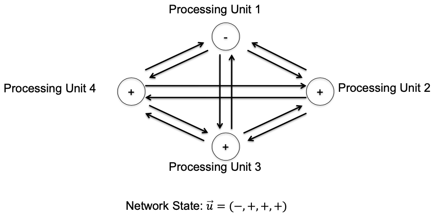
Connections
Processing units fully interconnected
Weights from unit $j$ to unit $i$: $T_{ij}$
No unit has a connection with itself $$ \forall i : \qquad T_{ii} = 0
$$Weights between a pair of units are symmetric $$ T_{ji} = T_{ij} $$
- Symmetric weights lead to the fact that the network will converge (relax in stable state)
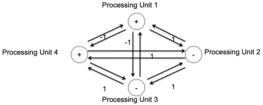
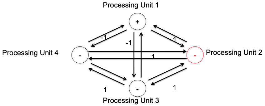
Example
Unit vector: $$ U = (+1, -1, -1, +1)^T $$ Weight matrix:
$$ T=\left(\begin{array}{cccc} T_{11} & T_{12} & T_{13} & T_{14} \\ T_{21} & T_{22} & T_{23} & T_{24} \\ T_{31} & T_{32} & T_{33} & T_{34} \\ T_{41} & T_{42} & T_{43} & T_{44} \end{array}\right) = \left(\begin{array}{cccc} 0 & -1 & -1 & +1 \\ -1 & 0 & +1 & -1 \\ -1 & +1 & 0 & -1 \\ +1 & -1 & -1 & 0 \end{array}\right) $$
Update Binary Unit
$$ u_i = \operatorname{sign}(\sum_{j} T_{ji} u_j) = \begin{cases} +1 & \text{if }\sum_{j} T_{ji} u_j \geq 0 \\ -1 & \text {otherwise } \end{cases} $$
- Evaluate the sum of the weighted inputs
- Set state $1$ if the sum is greater or equal $0$, else $-1$
Update Procedure
Network state is initialized in the beginning
Update
- Asynchronous: Update one unit at a time
- Synchronous: Update all nodes in parallel
Continue updating until the network state does not change anymore
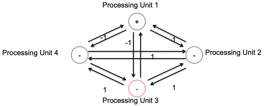
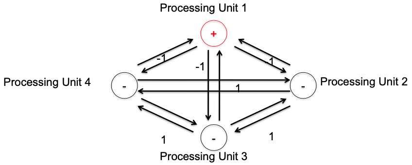
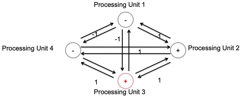
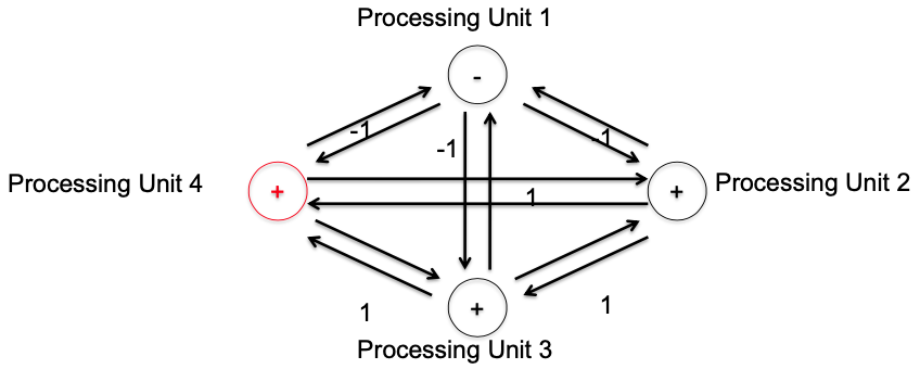
Example
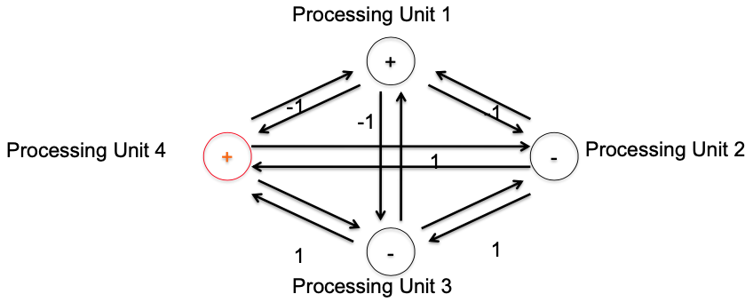
$$ u_4 = \operatorname{sign}(+1 \cdot (-1) + (-1) \cdot 1 + (-1) \cdot 1) = \operatorname{sign}(-3) = -1 $$
So the new state of unit 4 is $-$

Order of updating
Could be sequentially
Random order (Hopfield networks)
Same average update rate
Advantages in implementation
Advantages in function (equiprobable stable states)
Randomized asynchronous updating is a closer match to the biological neuronal nets
Energy function
Assign a numerical value to each possible state of the system (Lyapunov Function)
Corresponds to the “energy” of the net $$ \begin{aligned} E &= -\frac{1}{2} \sum_{j} \sum_{i \neq j} u_{i} T_{j i} u_{j} \\ &= -\frac{1}{2}U^T TU \end{aligned} $$
Proof on Convergence
Each updating step leads to lower or same energy in the net.
Let’s say only unit $j$ is updated at a time. Energy changes only for unit $j$ is $$ E_{j}=-\frac{1}{2} \sum_{i \neq j} u_{i}T_{j i} u_{j} $$ Given a change in state, the difference in Energy $E$ is $$ \begin{aligned} \Delta E_{j}&=E_{j_{n e w}}-E_{j_{o l d}} \\ &=-\frac{1}{2} \Delta u_{j} \sum_{i \neq j} u_{j} T_{j i} \end{aligned} $$
$$ \Delta u_{j}=u_{j_{n e w}}-u_{j_{o l d}} $$
Change from $-1$ to $1$: $$ \Delta u_{j}=2, \Sigma T_{j i} u_{i} \geq 0 \Rightarrow \Delta E_{j} \leq 0 $$
Change from $1$ to $-1$: $$ \Delta u_{j}=-2, \Sigma T_{j i} u_{i}<0 \Rightarrow \Delta E_{j}<0 $$
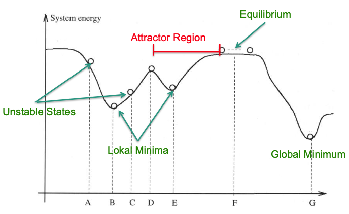
Stable States
Stable states are minima of the energy function
- Can be global or local minima
Analogous to finding a minimum in a mountainous terrain
Applications
Associative memory
Optimization
Limitations
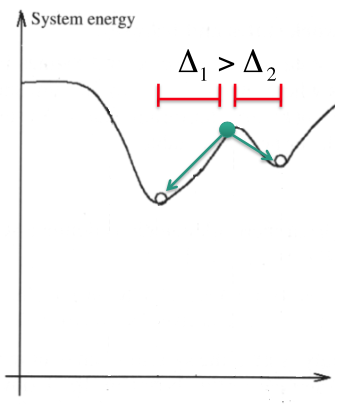
Found stable state (memory) is not guaranteed the most similar pattern to the input pattern
Not all memories are remembered with same emphasis (attractors region is not the same size)
Spurious States
Retrieval States
Reversed States
Mixture States: Any linear combination of an odd number of patterns
“Spinglass” states: Stable states that are no linear combination of stored patterns (occur when too many patterns are stored)
Efficiency
In a net of $N$ units, patterns of length $N$ can be stored
Assuming uncorrelated patterns, the capacity $C$ of a hopfield net is $$ C \approx 0.15N $$
- Tighter bound $$ \frac{N}{4 \ln N}<C<\frac{N}{2 \ln N} $$