Restricted Boltzmann Machines (RBMs)
Definition
Invented by Geoffrey Hinton, a Restricted Boltzmann machine is an algorithm useful for
- dimensionality reduction
- classification
- regression
- collaborative filtering
- feature learning
- topic modeling
Given their relative simplicity and historical importance, restricted Boltzmann machines are the first neural network we’ll tackle.
Structure
RBMs are shallow, two-layer neural nets that constitute the building blocks of deep-belief networks.
- The first layer of the RBM is called the visible, or input, layer.
- The second is the hidden layer.
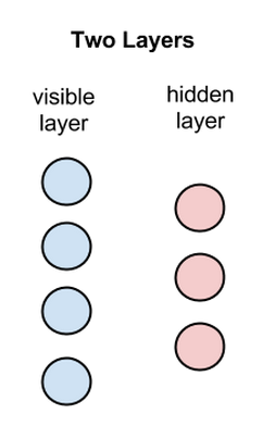
Each circle in the graph above represents a neuron-like unit called a node
Nodes are simply where calculations take place
Nodes are connected to each other across layers, but NO two nodes of the SAME layer are linked
$\to$ NO intra-layer communication (restriction in a restricted Boltzmann machine)
Each node is a locus of computation that processes input, and begins by making stochastic decisions about whether to transmit that input or not
Stochastic means “randomly determined”, and in this case, the coefficients that modify inputs are randomly initialized.
Each visible node takes a low-level feature from an item in the dataset to be learned.
- E.g., from a dataset of grayscale images, each visible node would receive one pixel-value for each pixel in one image. (MNIST images have 784 pixels, so neural nets processing them must have 784 input nodes on the visible layer.)
Forward pass
One input path
Now let’s follow that single pixel value, x, through the two-layer net. At node 1 of the hidden layer,
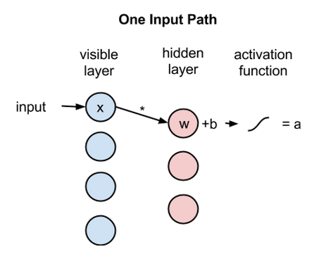
- x is multiplied by a weight and added to a so-called bias
- The result of those two operations is fed into an activation function, which produces the node’s output
activation f((weight w * input x) + bias b ) = output a
Weighted inputs combine
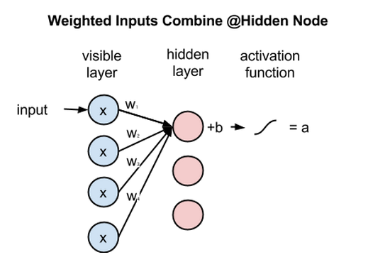
- Each x is multiplied by a separate weight
- The products are summed and added to a bias
- The result is passed through an activation function to produce the node’s output.
Because inputs from all visible nodes are being passed to all hidden nodes, an RBM can be defined as a symmetrical bipartite graph
- Symmetrical: each visible node is connected with each hidden node
- Bipartite: it has two parts, or layers, and the graph is a mathematical term for a web of nodes
Multiple inputs
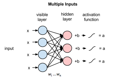
- At each hidden node, each input x is multiplied by its respective weight w.
- 12 weights altogether (4 input nodes x 3 hidden nodes)
- The weights between two layers will always form a matrix
- #rows = #input nodes
- #columns = #output nodes
- Each hidden node
- receives the four inputs multiplied by their respective weights
- The sum of those products is again added to a bias (which forces at least some activations to happen)
- The result is passed through the activation algorithm producing one output for each hidden node
Multiple hidden layers
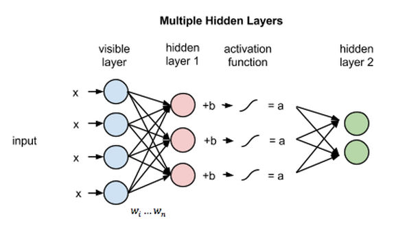
If these two layers were part of a deeper neural network, the outputs of hidden layer no. 1 would be passed as inputs to hidden layer no. 2, and from there through as many hidden layers as you like until they reach a final classifying layer.
(For simple feed-forward movements, the RBM nodes function as an autoencoder and nothing more.)
Reconstructions
In this section, we’ll focus on how they learn to reconstruct data by themselves in an unsupervised fashion, making several forward and backward passes between the visible layer and hidden layer no. 1 without involving a deeper network.
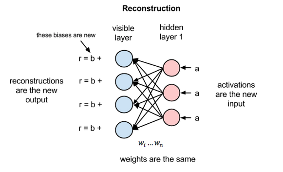
- The activations of hidden layer no. 1 become the input in a backward pass.
- They are multiplied by the same weights, one per internode edge, just as x was weight-adjusted on the forward pass.
- The sum of those products is added to a visible-layer bias at each visible node
- The output of those operations is a reconstruction; i.e. an approximation of the original input.
We can think of reconstruction error as the difference between the values of r and the input values, and that error is then backpropagated against the RBM’s weights, again and again, in an iterative learning process until an error minimum is reached.
Kullback Leibler Divergence
On its forward pass, an RBM uses inputs to make predictions about node activations, or the probability of output given a weighted x: p(a|x; w).
on its backward pass, an RBM is attempting to estimate the probability of inputs x given activations a, which are weighted with the same coefficients as those used on the forward pass: p(x|a; w)
Together, those two estimates will lead us to the joint probability distribution of inputs x and activations a, or p(x, a).
Reconstruction is making guesses about the probability distribution of the original input; i.e. the values of many varied points at once. And this is known as generative learning.
Imagine that both the input data and the reconstructions are normal curves of different shapes, which only partially overlap. To measure the distance between its estimated probability distribution and the ground-truth distribution of the input, RBMs use Kullback Leibler Divergence.
KL-Divergence measures the non-overlapping, or diverging, areas under the two curves
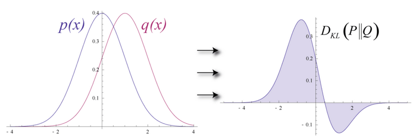
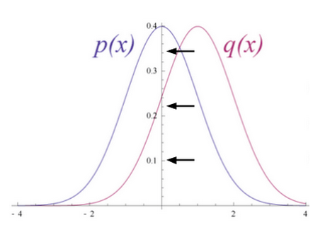
An RBM’s optimization algorithm attempts to minimize those areas so that the shared weights, when multiplied by activations of hidden layer one, produce a close approximation of the original input. By iteratively adjusting the weights according to the error they produce, an RBM learns to approximate the original data.
The learning process looks like two probability distributions converging, step by step.
Probabilistic View
For example, image datasets have unique probability distributions for their pixel values, depending on the kind of images in the set.
Assuming an RBM that was only fed images of elephants and dogs, and which had only two output nodes, one for each animal.
- The question the RBM is asking itself on the forward pass is: Given these pixels, should my weights send a stronger signal to the elephant node or the dog node?
- The question the RBM asks on the backward pass is: Given an elephant, which distribution of pixels should I expect?
That’s joint probability: the simultaneous probability of x given a and of a given x, expressed as the shared weights between the two layers of the RBM.
The process of learning reconstructions is, in a sense, learning which groups of pixels tend to co-occur for a given set of images. The activations produced by nodes of hidden layers deep in the network represent significant co-occurrences; e.g. “nonlinear gray tube + big, floppy ears + wrinkles” might be one.