Recurrent Neural Networks
Overview
- Specifically designed for long-range dependency
- 💡 Main idea: connecting the hidden states together within a layer
Simple RNNs
Elman Networks
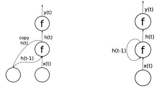
- The output of the hidden layer is used as input for the next time step
- They use a copy mechanism. Previous state of H copied into next iteration of net
- Do NOT really have true recurrence, no backpropagation through time
Jordan Nets
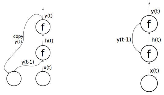
- Same Copy Mechanisms as Elman Networks, but from Output Layer
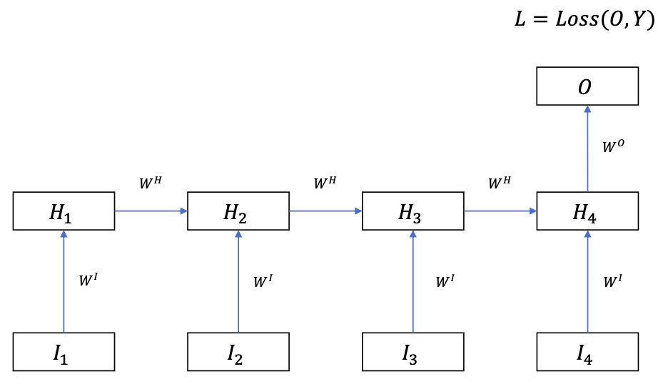
RNN Structure
 $$
H\_{t}=f\_{a c t}\left(W^{H} H\_{t-1}+W^{X} X\_{t}+b\right)
$$
$$
H\_{t}=f\_{a c t}\left(W^{H} H\_{t-1}+W^{X} X\_{t}+b\right)
$$- $f\_{act}$: activation function (sigmoid, tanh, ReLU … )
- Inside the bracket: a linear “voting” combination between the memory $H\_{t-1}$ and input $X\_t$
Learning in RNNs: BPTT
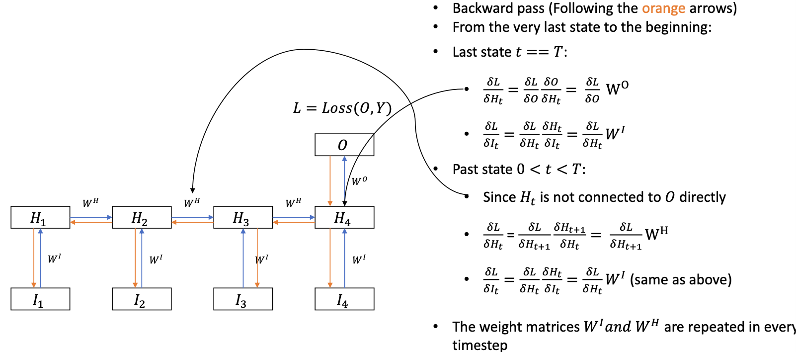
One-to-One RNN
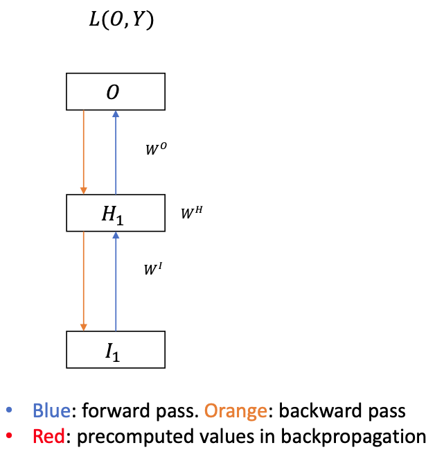
Identical to a MLP
$W^H$ is non-existent or an identity function
Backprop (obviously) like an MLP
- $\frac{\delta L}{\delta O}$ is directly computed from $L(O, Y)$
(Red terms are precomputed values in backpropagation)
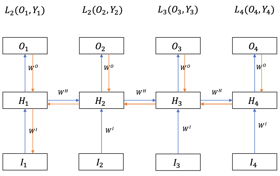
Many-to-One RNN
Often used to sequence-level classification
For example:
- Movie review sentiment analysis
- Predicting blood type from DNA
Input: sequence $I \in \mathbb{R}^{T \times D\_I}$
Output: vector $O \in \mathbb{R}^{D\_O}$
Backprop
- The gradient signal is backpropagated through time by the recurrent connections
- Shared weights: the weight matrices are duplicated over the time dimension
- In each time step, the weights $\theta = (W^H, W^I, W^O)$ establishes a multi-layer perceptron.
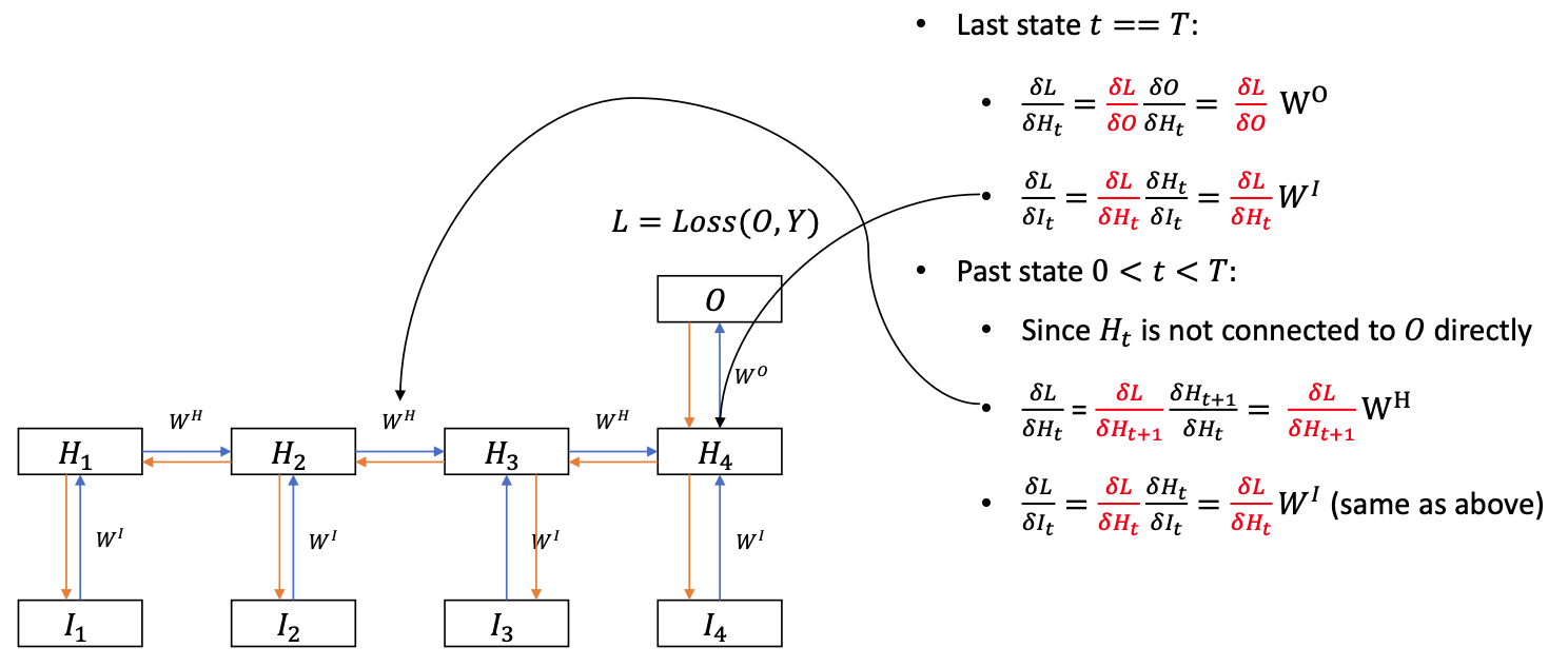
- The gradients are summed up over time $$ \begin{aligned} \frac{\delta L}{\delta W^{I}} &=\frac{\delta L}{\delta W\_{1}^{I}}+\frac{\delta L}{\delta W_{2}^{I}}+\cdots+\frac{\delta L}{\delta W\_{T}^{I}} \\\\ \\\\ \frac{\delta L}{\delta W^{H}} &=\frac{\delta L}{\delta W\_{1}^{H}}+\frac{\delta L}{\delta W\_{2}^{H}}+\cdots+\frac{\delta L}{\delta W\_{T-1}^{H}} \end{aligned} $$
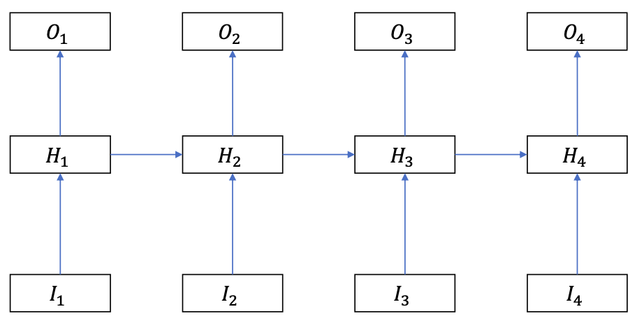
Many-to-Many RNN
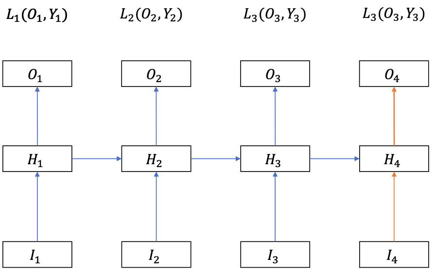
The inputs and outputs have the same number of elements
Example
- Auto-regressive models
- Character generation model
- Pixel models
Backprop
Loss function
$$ L = L\_1 + L\_2 + \cdots + L\_T $$$H\_t$ can not change $O\_{k
(Because we cannot change the past so the terms with $i < t$ can be omitted)
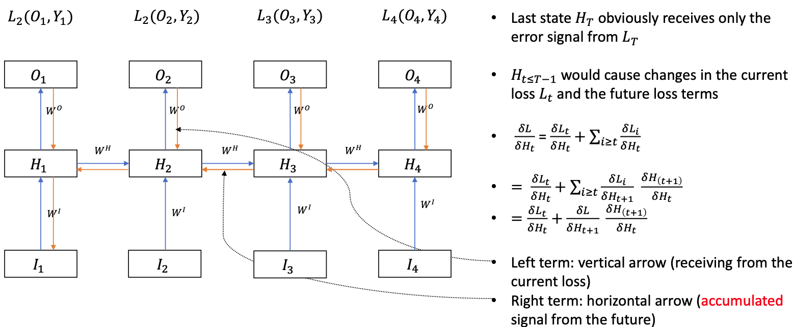
After getting the $\frac{\delta L}{\delta H\_t}$ terms, we can compute the necessary gradients for $\frac{\delta L}{\delta W^{O}}, \frac{\delta L}{\delta W^{H}}$ and $\frac{\delta L}{\delta W^{I}}$
For shared weights $W^O$, apply the same principle in the Many-to-One RNN.
One-to-Many RNN
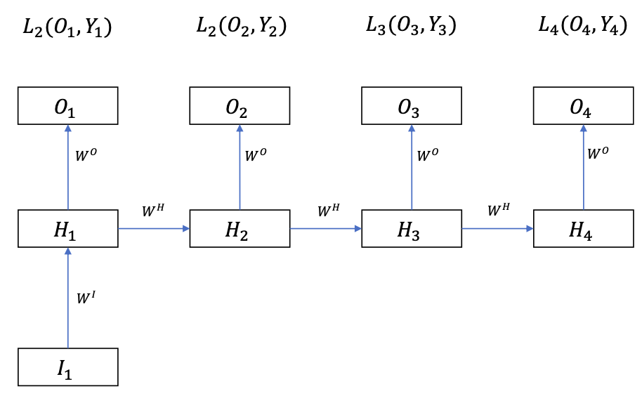
More rarely seen than Many-to-One
For example:
- Image description generation
- Music generation
Input: vector $I \in \mathbb{R}^{D\_{I}}$
Output: sequence $O \in R^{T \times D\_{O}}$
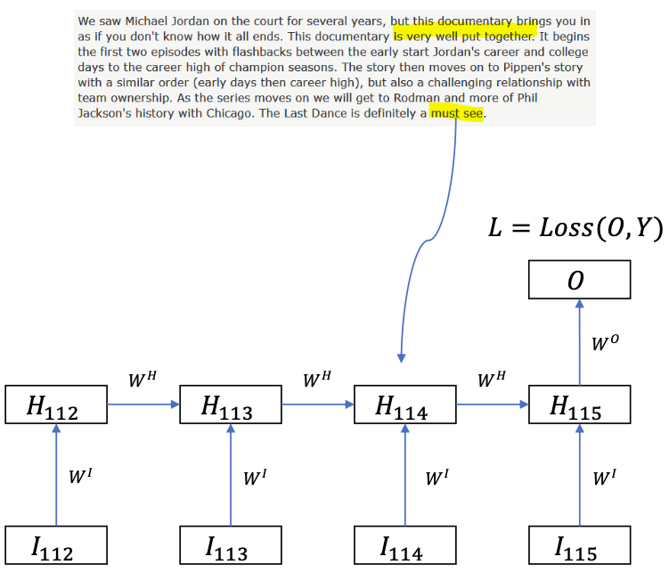
Problem of BPTT
 $$
\begin{array}{l}
\frac{\delta L}{\delta H\_{114}}=\frac{\delta L}{\delta H\_{115}} \frac{\delta H\_{115}}{\delta H\_{114}} \\\\ \\\\
\frac{\delta L}{\delta H_{113}}=\frac{\delta L}{\delta H\_{115}} \frac{\delta H\_{115}}{\delta H\_{114}} \frac{\delta H\_{114}}{\delta H\_{113}}=W^{O} f^{\prime}\left(H\_{115}\right) W^{H} f^{\prime}\left(H\_{114}\right) W^{H}
\end{array}
$$
If we wand to send signals back to step 50:
$$
\begin{aligned}
\frac{\delta L}{\delta H\_{50}} &=\frac{\delta L}{\delta H\_{115}} \frac{\delta H\_{115}}{\delta H\_{114}} \ldots \frac{\delta H\_{51}}{\delta H\_{50}} \\\\ \\\\
&=W^{O} f^{\prime}\left(H\_{115}\right) W^{H} f^{\prime}\left(H\_{114}\right) W^{H} f^{\prime}\left(H\_{113}\right) W^{H} \ldots
\end{aligned}
$$
65 times of repetition for $f^{\prime}\left(H\_{115}\right) W^{H}$!!! 😱😱😱
$$
\begin{array}{l}
\frac{\delta L}{\delta H\_{114}}=\frac{\delta L}{\delta H\_{115}} \frac{\delta H\_{115}}{\delta H\_{114}} \\\\ \\\\
\frac{\delta L}{\delta H_{113}}=\frac{\delta L}{\delta H\_{115}} \frac{\delta H\_{115}}{\delta H\_{114}} \frac{\delta H\_{114}}{\delta H\_{113}}=W^{O} f^{\prime}\left(H\_{115}\right) W^{H} f^{\prime}\left(H\_{114}\right) W^{H}
\end{array}
$$
If we wand to send signals back to step 50:
$$
\begin{aligned}
\frac{\delta L}{\delta H\_{50}} &=\frac{\delta L}{\delta H\_{115}} \frac{\delta H\_{115}}{\delta H\_{114}} \ldots \frac{\delta H\_{51}}{\delta H\_{50}} \\\\ \\\\
&=W^{O} f^{\prime}\left(H\_{115}\right) W^{H} f^{\prime}\left(H\_{114}\right) W^{H} f^{\prime}\left(H\_{113}\right) W^{H} \ldots
\end{aligned}
$$
65 times of repetition for $f^{\prime}\left(H\_{115}\right) W^{H}$!!! 😱😱😱Assuming network is univariate $W^H$ has one element $w$ and $f$ is either ReLU or linear
If $w = 1.1$: $\frac{\delta L}{\delta H_{50}}=117$
If $w = 0.9$: $\frac{\delta L}{\delta H_{50}}=0.005$
In general
if the maximum eigenvalue of $W^H > 1$: $\frac{\delta L}{\delta H_{T}}$ is likely to explode (Gradient explosion)
More see: Exploding Gradient Problem
- Solution
- Gradient clipping
- Weight regularization
- Solution
if the maximum eigenvalue of $W^H < 1$: $\frac{\delta L}{\delta H_{T}}$ is likely to vanish (Gradient vanishing)
- small gradients make the RNN unable to learn the important features to solve the problem
Gradient clipping
Simple solution for gradient exploding
Rescale gradients so that their norm is at most a particular value.
- Clip the gradient $g = \frac{\delta L}{\delta w}$ so
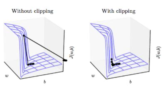
With gradient clipping, pre-determined gradient threshold be introduced, and then gradients norms that exceed this threshold are scaled down to match the norm. This prevents any gradient to have norm greater than the threshold and thus the gradients are clipped.
More see: Gradient Clipping