K Nearest Neighbors
Non-parametric Methods
- Store all the training data
- Use the training data for doing predictions
- Do NOT adapt parameters
- Often referred to as instance-based methods
👍 Advantages
- Complexity adapts to training data
- Very fast at training
👎 Disadvantages
- Slow for prediction
- Hard to use for high-dimensional input
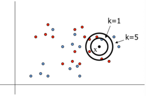
$k$-Nearest Neighbour Classifiers
To classify a new input vector $x,$
- Examine the $k$-closest training data points to $x$ (comman values for $k$: $k=3$, $k=5$)
- Assign the object to the most frequently occurring class
🤔 When to consider?
- Can measure distances between data-points
- Less than 20 attributes per instance
- Lots of training data
👍 Advantages
- Training is very fast
- Learn complex target functions
- Similar algorithm can be used for regression
- High accuracy
- Insensitive to outliers
- No assumptions about data
👎 Disadvantages
- Computationally expensive
- requires a lot of memory
Decision Boundaries
- The nearest neighbour algorithm does NOT explicitly compute decision boundaries.
- The decision boundaries form a subset of the Voronoi diagram for the training data.
- The more data points we have, the more complex the decision boundary can become
Distance Metrics
Most common distance metric: Euclidean distance (ED)
$$ d(\boldsymbol{x}, \boldsymbol{y})=\|\boldsymbol{x}-\boldsymbol{y}\|=\sqrt{\left(\sum_{k=1}^{d}\left(\boldsymbol{x}_{k}-\boldsymbol{y}_{k}\right)^{2}\right)} $$makes sense when different features are commensurate; each is variable measured in the same units.
If the units are different (e.g.. length and weight), data needs to be normalised (resulting input dimensions are zero mean, unit variance)
$$ \tilde{\boldsymbol{x}}=(\boldsymbol{x}-\boldsymbol{\mu}) \oslash \boldsymbol{\sigma} $$- $\mu$: Mean
- $\sigma$: Standard deviation
- $\oslash$: element-wise division
Another distance metrics:
Cosine Distance: Good for documents, images $$ d(\boldsymbol{x}, \boldsymbol{y})=1-\frac{\boldsymbol{x}^{T} \boldsymbol{y}}{\|\boldsymbol{x}\|\|\boldsymbol{y}\|} $$
Hamming Distance: For string data / categorical features $$ d(\boldsymbol{x}, \boldsymbol{y})=\sum_{k=1}^{d}\left(\boldsymbol{x}_{k} \neq \boldsymbol{y}_{k}\right) $$
Manhattan Distance: Coordinate-wise distance $$ d(\boldsymbol{x}, \boldsymbol{y})=\sum_{k=1}^{d}\left|\boldsymbol{x}_{k}-\boldsymbol{y}_{k}\right| $$
Mahalanobis Distance: Normalized by the sample covariance matrix – unaffected by coordinate transformations $$ d(\boldsymbol{x}, \boldsymbol{y})=\|\boldsymbol{x}-\boldsymbol{y}\|_{\Sigma^{-1}}=\sqrt{(\boldsymbol{x}-\boldsymbol{y})^{T} \boldsymbol{\Sigma}^{-1}(\boldsymbol{x}-\boldsymbol{y})} $$