Smoothing

To keep a language model from assigning zero probability to these unseen events, we’ll have to shave off a bit of probability mass from some more frequent events and give it to the events we’ve never seen.

Laplace smoothing (Add-1 smoothing)

💡 Idea: add one to all the bigram counts, before we normalize them into probabilities.

• does not perform well enough to be used in modern n-gram models 🤪, but
• usefully introduces many of the concepts
• gives a useful baseline
• a practical smoothing algorithm for other tasks like text classification

Unsmoothed maximum likelihood estimate of the unigram probability of the word $w_i$: its count $c_i$ normalized by the total number of word tokens $N$

Laplace smoothed:

• Merely adds one to each count
• Since there are $V$ words in the vocabulary and each one was incremented, we also need to adjust the denominator to take into account the extra $V$ observations.

Adjust count $c^*$

• easier to compare directly with the MLE counts and can be turned into a probability like an MLE count by normalizing by $N$

  $\frac{c_I^*}{N} = \left(c_{i}+1\right) \frac{N}{N+V} \cdot \frac{1}{N} =\frac{c_{i}+1}{N+V} = P_{\text {Laplace}}\left(w_{i}\right)$

Another aspect of smoothing

A related way to view smoothing is as discounting (lowering) some non-zero counts in order to get the probability mass that will be assigned to the zero counts.

Thus, instead of referring to the discounted counts $c^{\*}$, we might describe a smoothing algorithm in terms of a relative discount $d_c$

(the ratio of the discounted counts to the original counts)

Example

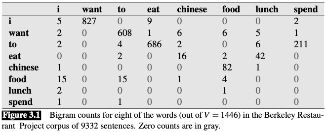
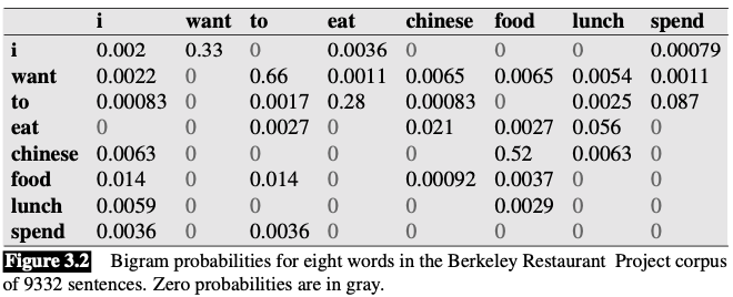
Smooth the Berkeley Restaurant Project bigrams

• Original(unsmoothed) bigram counts and probabilities

  

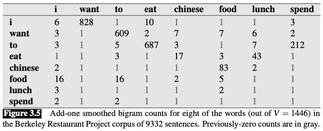
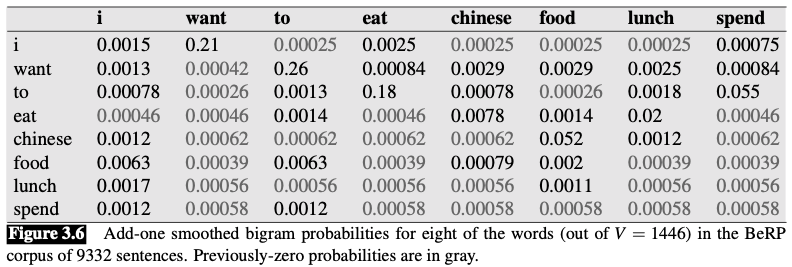
• Add-one smoothed counts and probabilities

  

Computation:

• Recall: normal bigram probabilities are computed by normalizing each row of counts by the unigram count

  $$P\left(w_{n} | w_{n-1}\right)=\frac{C\left(w_{n-1} w_{n}\right)}{C\left(w_{n-1}\right)}$$

• add-one smoothed bigram: augment the unigram count by the number of total word types in the vocabulary

  $$P_{\text {Laplace }}^{*}\left(w_{n} | w_{n-1}\right)=\frac{C\left(w_{n-1} w_{n}\right)+1}{\sum_{w}\left(C\left(w_{n-1} w\right)+1\right)}=\frac{C\left(w_{n-1} w_{n}\right)+1}{C\left(w_{n-1}\right)+V}$$

• It is often convenient to reconstruct the count matrix so we can see how much a smoothing algorithm has changed the original counts.

  $$c^{*}\left(w_{n-1} w_{n}\right)=\frac{\left[C\left(w_{n-1} w_{n}\right)+1\right] \times C\left(w_{n-1}\right)}{C\left(w_{n-1}\right)+V}$$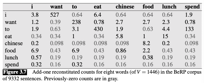

  

Add-one smoothing has made a very big change to the counts.

• $C(\text{want to})$ changed from 609 to 238
• $P(to|want)$ decreases from .66 in the unsmoothed case to .26 in the smoothed case
• The discount $d$ (the ratio between new and old counts) shows us how strikingly the counts for each prefix word have been reduced
  • the discount for the bigram want to is .39
  • the discount for Chinese food is .10

The sharp change in counts and probabilities occurs because too much probability mass is moved to all the zeros.

Add-k smoothing

Instead of adding 1 to each count, we add a fractional count $k$

• $k$: can be chosen by optimizing on a devset (validation set)

Add-k smoothing

• useful for some tasks (including text classification)
• still doesn’t work well for language modeling, generating counts with poor variances and often inappropriate discounts 🤪

Backoff and interpolation

Sometimes using less context is a good thing, helping to generalize more for contexts that the model hasn’t learned much about.

Backoff

💡 “Back off” to a lower-order n-gram if we have zero evidence for a higher-order n-gram

• If the n-gram we need has zero counts, we approximate it by backing off to the (n-1)-gram. We continue backing off until we reach a history that has some counts.
  • we use the trigram if the evidence is sufficient, otherwise we use the bigram, otherwise the unigram.

Katz backoff

• Rely on a discounted probability $P^*$ if we’ve seen this n-gram before (i.e., if we have non-zero counts)

  • We have to discount the higher-order n-grams to save some probability mass for the lower order n-grams

    if the higher-order n-grams aren’t discounted and we just used the undiscounted MLE probability, then as soon as we replaced an n-gram which has zero probability with a lower-order n-gram, we would be adding probability mass, and the total probability assigned to all possible strings by the language model would be greater than 1!

• Otherwise, we recursively back off to the Katz probability for the shorter-history (n-1)-gram.

$\Rightarrow$ The probability for a backoff n-gram $P_{\text{BO}}$ is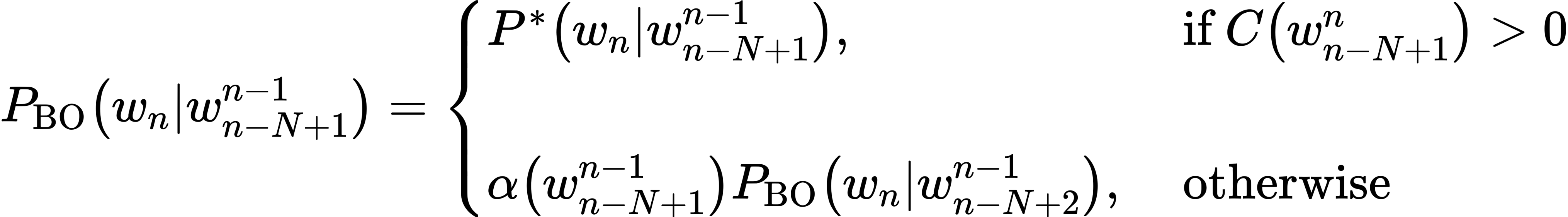

• $P^*$: discounted probability
• $\alpha$: a function to distribute the discounted probability mass to the lower order n-grams

Interpolation

💡 Mix the probability estimates from all the n-gram estimators, weighing and combining the trigram, bigram, and unigram counts.

In simple linear interpolation, we combine different order n-grams by linearly interpolating all the models. I.e., we estimate the trigram probability $P\left(w_{n} | w_{n-2} w_{n-1}\right)$ by mixing together the unigram, bigram, and trigram probabilities, each weighted by a $\lambda$

s.t.

In a slightly more sophisticated version of linear interpolation, each $\lambda$ weight is computed by conditioning on the context.

• If we have particularly accurate counts for a particular bigram, we assume that the counts of the trigrams based on this bigram will be more trustworthy, so we can make the $λ$s for those trigrams higher and thus give that trigram more weight in the interpolation.

How to set $\lambda$s?

Learn from a held-out corpus

• Held-out corpus: an additional training corpus that we use to set hyperparameters like these $λ$ values, by choosing the $λ$ values that maximize the likelihood of the held-out corpus.
• We fix the n-gram probabilities and then search for the $λ$ values that give us the highest probability of the held-out set
  • Common method: EM algorithm

Kneser-Ney Smoothing 👍

One of the most commonly used and best performing n-gram smoothing methods 👏

Based on absolute discounting

• subtracting a fixed (absolute) discount $d$ from each count.
• 💡 Intuition:
  • since we have good estimates already for the very high counts, a small discount d won’t affect them much
  • It will mainly modify the smaller counts, for which we don’t necessarily trust the estimate anyway

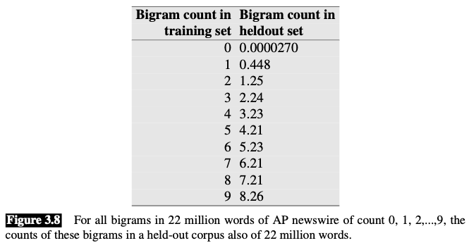
Except for the held-out counts for 0 and 1, all the other bigram counts in the held-out set could be estimated pretty well by just subtracting 0.75 from the count in the training set! In practice this discount is actually a good one for bigrams with counts 2 through 9.

The equation for interpolated absolute discounting applied to bigrams:

• First term: discounted bigram
  • We could just set all the $d$ values to .75, or we could keep a separate discount value of 0.5 for the bigrams with counts of 1.
• Second term: unigram with an interpolation weight $\lambda$

Kneser-Ney discounting augments absolute discounting with a more sophisticated way to handle the lower-order unigram distribution.

Sophisticated means: Instead of $P(w)$ which answers the question “How likely is $w$?”, we’d like to create a unigram model that we might call $P\_{\text{CONTINUATION}}$, which answers the question “How likely is w to appear as a novel continuation?”

How can we estimate this probability of seeing the word $w$ as a novel continuation, in a new unseen context?

💡 The Kneser-Ney intuition: base our $P\_{\text{CONTINUATION}}$ on the number of different contexts word $w$ has appeared in (the number of bigram types it completes).

• Every bigram type was a novel continuation the first time it was seen.
• We hypothesize that words that have appeared in more contexts in the past are more likely to appear in some new context as well.

The number of times a word $w$ appears as a novel continuation can be expressed as:

To turn this count into a probability, we normalize by the total number of word bigram types:

An equivalent formulation based on a different metaphor is to use the number of word types seen to precede $w$, normalized by the number of words preceding all words,

The final equation for Interpolated Kneser-Ney smoothing for bigrams is:

• $λ$: normalizing constant that is used to distribute the probability mass

  $$\lambda(w_{i-1})=\frac{d}{\sum_{v} C(w_{i-1} v)}|\{w: C(w_{i-1} w)>0\}|$$
  • First term: normalized discount
  • Second term: the number of word types that can follow $w_{i-1}$. or, equivalently, the number of word types that we discounted (i.e., the number of times we applied the normalized discount.)

The general recursive formulation is

• $C_{KN}$: depends on whether we are counting the highest-order n-gram being interpolated or one of the lower-order n-grams

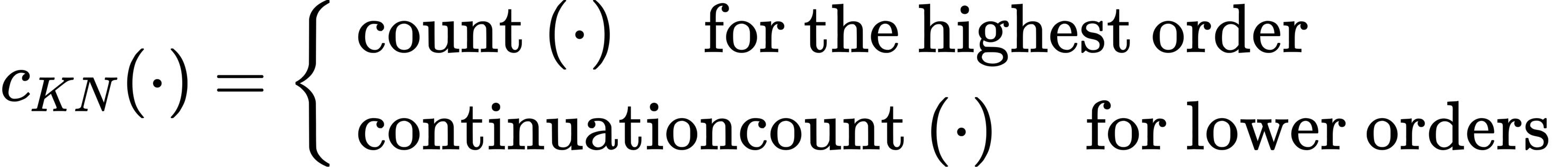
  • $\operatorname{continuationcount}(\cdot)$: the number of unique single word contexts for $\cdot$

At the termination of the recursion, unigrams are interpolated with the uniform distribution

• $\varepsilon$: empty string