Reapproximation von Dichten
4 cases
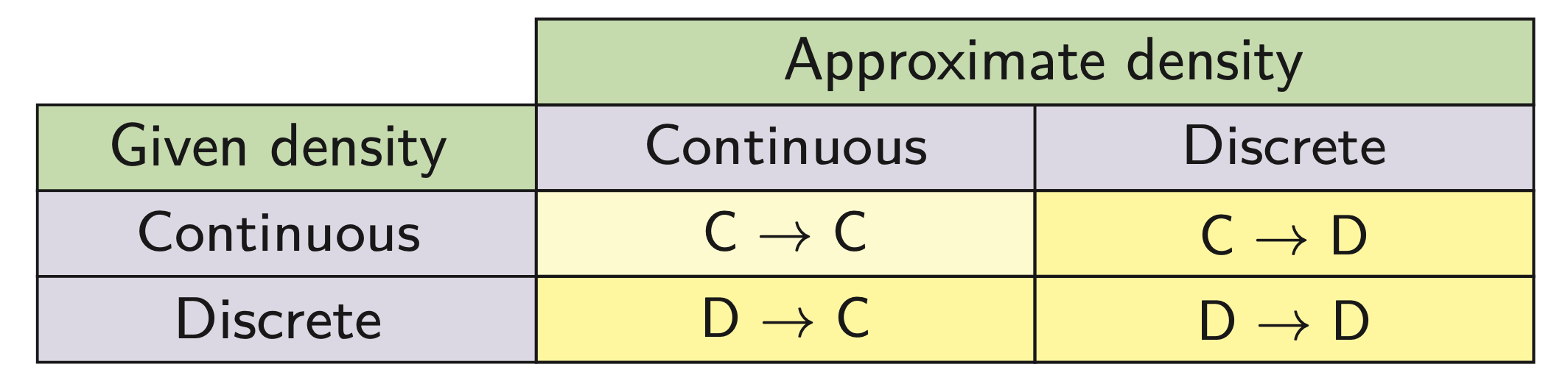
Examples for reapproximation
Continuous → continuous: Gaussian mixture reduction
Continuous → discrete: deterministic sampling, i.e., replacing a continuous density with Dirac mixture
Discrete → continuous: density estimation, i.e., finding a continuous density representing a set of given samples
Discrete → discrete: Dirac mixture reduction
Challenge: Three cases involving discrete densities
Continuous → continuous case: Use standard distance measures, e.g. integral squared distance (ISD)
Discrete densities prohibit use of standard distance measures
Here we focus on continuous → discrete Reapproximation
Given: Continuous density $\tilde{f}(\underline{x})$
Deterministic sampling, i.e., approximation with Dirac mixture
Definition of Dirac mixture with $L$ components
$$ f(\underline{x})=\sum_{i=1}^{L} w_{i} \cdot \delta\left(\underline{x}-\underline{\hat{x}}_{i}\right) $$- Weights $w_{i}>0, \displaystyle \sum_{i=1}^{L} w_{i}=1$
- $\underline{x}_i$: locations / samples
🎯 Goal: Systematic approximation of given continuous density
Application examples
Mapping of random variables through nonlinear functions
Sample-based fusion and estimation (UKF)
Univariate Case (1D)
Synthesis
Instead of comparing densities $\tilde{f}(x), f(x)$, we compare cumulative distribution functions (CDFs) $\tilde{F}(x), F(x)$
CDF of $f(x)$:
$$ F(x)=P(\boldsymbol{x} \leq x)=\int_{-\infty}^{x} f(u) \mathrm{d} u $$This definition is unique, as other definition $\bar{F}(x)=P(\boldsymbol{x}>x)$ is dependent
$$ \begin{aligned} \bar{F}(x)=&P(\boldsymbol{x}>x) \\ &=\int_{x}^{\infty} f(u) d u \\ &=1-\int_{-\infty}^{x} f(u) d u \\ &=1-P(\boldsymbol{x} \leq x) \\ &=1-F(x) \end{aligned} $$Example
Dirac mixture density
$$ f(x, \underline{\hat{x}})=\sum_{i=1}^{L} w_{i} \delta\left(x-\hat{x}_{i}\right) $$Dirac mixture cumulative distribution
$$ F(x, \underline{\hat{x}})=\sum_{i=1}^{L} w_{i} \mathrm{H}\left(x-\hat{x}_{i}\right) \text { with } \mathrm{H}(x)=\int_{-\infty}^{x} \delta(t) \mathrm{d} t= \begin{cases}0 & x<0 \\ \frac{1}{2} & x=0 \\ 1 & x>0\end{cases} $$with the Dirac position
$$ \underline{\hat{x}}=\left[\hat{x}_{1}, \hat{x}_{2}, \ldots, \hat{x}_{L}\right]^{\top} $$
CDF of $\tilde{f}(x)$ follows analogously:
$$ \tilde{F}(x)=\int_{-\infty}^{x} \tilde{f}(u) \mathrm{d} u $$Example
Gaussian density:
$$ \tilde{f}(x)=\frac{1}{\sqrt{2 \pi}} \exp \left(-\frac{1}{2} x^{2}\right) $$$\Rightarrow$ Gaussian cumulative distribution:
$$ \tilde{F}(x)=\frac{1}{2}\left(1+\operatorname{erf}\left(\frac{x}{\sqrt{2}}\right)\right) $$
We compare $\tilde{F}(x), F(x)$ use Cramér–von Mises distance:
$$ D(\underline{\hat{x}})=\int_{\mathbb{R}}(\tilde{F}(x)-F\left(x, \underline{\hat{x}})\right)^{2} \mathrm{~d} x $$Minimization of Cramér–von Mises distance
Gradient of the distance measure $D(\underline{\hat{x}})$:
$$ \underline{G}(\underline{\hat{x}})=\nabla D(\underline{\hat{x}})=\frac{\partial D(\underline{\hat{x}})}{\partial \underline{\hat{x}}}=\left[\frac{\partial D(\underline{\hat{x}})}{\partial \hat{x}_{1}}, \frac{\partial D(\underline{\hat{x}})}{\partial \hat{x}_{2}}, \ldots, \frac{\partial D(\underline{\hat{x}})}{\partial \hat{x}_{L}}\right]^{\top} $$with
$$ \frac{\partial D(\underline{\hat{x}})}{\partial \hat{x}_{i}}=2 w_{i} \int_{-\infty}^{\infty}[\tilde{F}(t)-F(t, \underline{\hat{x}})] \delta\left(t-\hat{x}_{i}\right) \mathrm{d} t $$or
$$ \frac{\partial D(\underline{\hat{x}})}{\partial \hat{x}_{i}}=2 w_{i}\left[\tilde{F}\left(\hat{x}_{i}\right)-F\left(\hat{x}_{i}, \underline{\hat{x}}\right)\right] \text { with } F\left(\hat{x}_{i}, \underline{\hat{x}}\right)=\sum_{j=1}^{L} w_{j} \mathrm{H}\left(\hat{x}_{i}-\hat{x}_{j}\right) $$The Hesse matrix is
$$ \mathbf{H}(\underline{x})=\operatorname{diag}\left(\left[\frac{\partial^{2} D(\underline{\hat{x}})}{\partial \hat{x}_{1}^{2}}, \frac{\partial^{2} D(\underline{\hat{x}})}{\partial \hat{x}_{2}^{2}}, \ldots, \frac{\partial^{2} D(\underline{\hat{x}})}{\partial \hat{x}_{L}^{2}}\right]\right) $$with
$$ \frac{\partial^{2} D(\underline{\hat{x}})}{\partial \hat{x}_{i}^{2}}=2 w_{i} \tilde{f}\left(\hat{x}_{i}\right) $$Sorted Locations & Equal Weights
When location vector $\underline{\hat{x}}$ is sorted, i.e., $\hat{x}_{1}<\hat{x}_{2}<\ldots<\hat{x}_{L}$ , we obtain
$$ H\left(\hat{x}_{i}-\hat{x}_{j}\right)= \begin{cases} 0 & i < j \\ \frac{1}{2} & i=j \\ 1 & i > j \end{cases} $$Cumulative distribution can be simplified
$$ F\left(\hat{x}_{i}, \underline{\hat{x}}\right)=\frac{w_{i}}{2}+\sum_{j=1}^{i-1} w_{j} $$When samples are equally weighted (i.e. $w_i = \frac{1}{L}$), we get
$$ F(\hat{x}_{i}, \underline{\hat{x}}) = \frac{1}{2L} + \frac{i-1}{L} = \frac{2i - 1}{2L} \qquad i = 1, \dots, L $$Analytic solutions (possible in some special cases)
$$ \tilde{F}\left(\hat{x}_{i}\right)-F\left(\hat{x}_{i}, \underline{\hat{x}}\right)=0 \Rightarrow \hat{x}_{i}=\tilde{F}^{-1}(\frac{2 i-1}{2 L}) \qquad i=1, \ldots, L $$E.g. Gaussian distribution:
$$ \tilde{F}^{-1}(x)=\sqrt{2} \operatorname{erfinv}((2 i-1) /(2 L)) $$
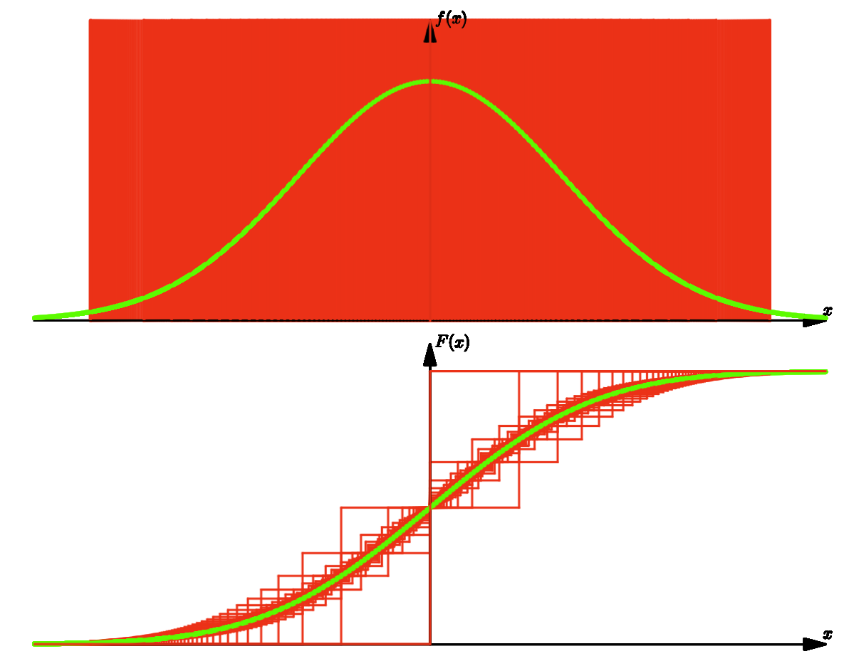
Example: DMA of standard Normal Distribution
With increasing number of Dirac functions, the CDF can be well approximated.
General Optimization
In general: Minimum of $D(\underline{\hat{x}})$ is obtained iteratively using Newton’s method
$$ \Delta \underline{\hat{x}}=-\mathbf{H}^{-1}(\underline{\hat{x}}) \underline{G}(\underline{\hat{x}}) $$with
$$ \underline{G}(\underline{\hat{\hat{x}}})=\left[\frac{\partial D(\underline{\hat{x}})}{\partial \hat{x}_{1}}, \frac{\partial D(\underline{\hat{x}})}{\partial \hat{x}_{2}}, \ldots, \frac{\partial D(\underline{\hat{x}})}{\partial \hat{x}_{L}}\right]^{\top} $$and
$$ \frac{\partial D(\underline{\hat{x}})}{\partial \hat{x}_{i}}=2 w_{i}\left[\tilde{F}\left(\hat{x}_{i}\right)-F\left(\hat{x}_{i}, \underline{\hat{x}}\right)\right] $$The Hessian $\mathbf{H}(\underline{x})$ is given by
$$ \mathbf{H}(\underline{\hat{x}})=2 \operatorname{diag}\left(\left[w_{1} \tilde{f}\left(\hat{x}_{1}\right), w_{2} \tilde{f}\left(\hat{x}_{2}\right), \ldots, w_{L} \tilde{f}\left(\hat{x}_{L}\right)\right]\right) $$The resulting Newton step:
$$ \Delta \underline{\hat{x}}=-\left[\frac{\tilde{F}\left(\hat{x}_{1}\right)-F\left(\hat{x}_{1}, \underline{\hat{x}}\right)}{\tilde{f}\left(\hat{x}_{1}\right)}, \frac{\tilde{F}\left(\hat{x}_{2}\right)-F\left(\hat{x}_{2}, \underline{\hat{x}}\right)}{\tilde{f}\left(\hat{x}_{2}\right)}, \ldots, \frac{\tilde{F}\left(\hat{x}_{L}\right)-F\left(\hat{x}_{L}, \underline{\hat{x}}\right)}{\tilde{f}\left(\hat{x}_{L}\right)}\right]^{\top} $$Extension to Multivariate Distributions
Extension to multivariate case is not trivial
- Less nice properties of multivariate cumulative distributions 🤪
Distinguish several classes of multivariate methods
- Methods that generalize concept of CDF
- Methods that perform reduction to univariate case
- Kernel-based methods
- Continuous flow between density approximations
Challenge of Multivariate Cumulative Distributions
Definition for 2D:
$$ F(u, v)=\int_{-\infty}^{u} \int_{-\infty}^{v} f(x, y) d x d y $$However, $F(u, v)$ is asymmetric and definition is not unique.
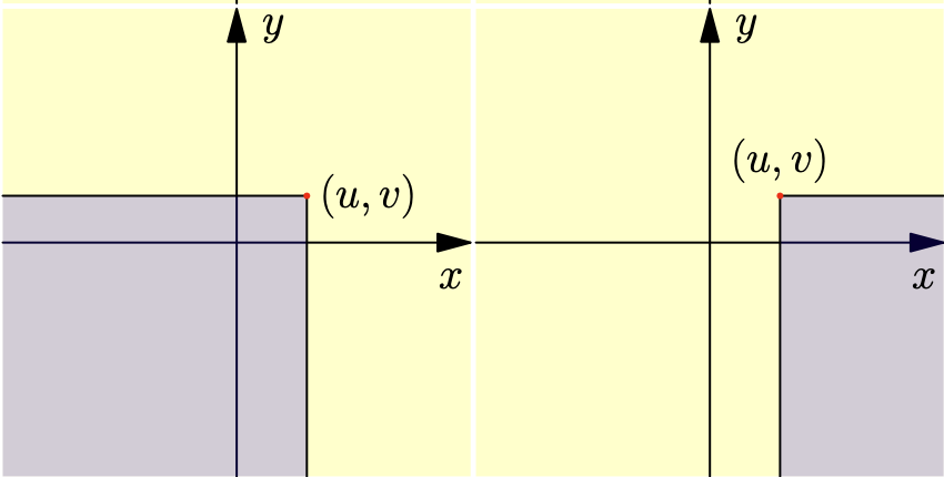
Alternative definitions:
$$ \begin{aligned} &F(u, v)=\int_{-\infty}^{u} \int_{v}^{\infty} f(x, y) d x d y \\ &F(u, v)=\int_{u}^{\infty} \int_{v}^{\infty} f(x, y) d x d y \\ &F(u, v)=\int_{u}^{\infty} \int_{-\infty}^{v} f(x, y) d x d y \end{aligned} $$- Three CDFs are independent, forth is dependent.
For general $N$–dimensional random vectors: $2^N$ different variants,, $2^N - 1$ are independent
$\rightarrow$ exponentially complex!
- Use in statistical tests difficult
- Results differ depending on variant
Thus, we require generalization of concept of CDF. 💪
Localized Cumulative Distributions (LCDs)
Univariate case (1D)
💡 Key idea
- Compare local probability masses of $\tilde{f}(x)$ and $f(x)$
- Integrate over intervals at all positions $m$ and all widths $b$
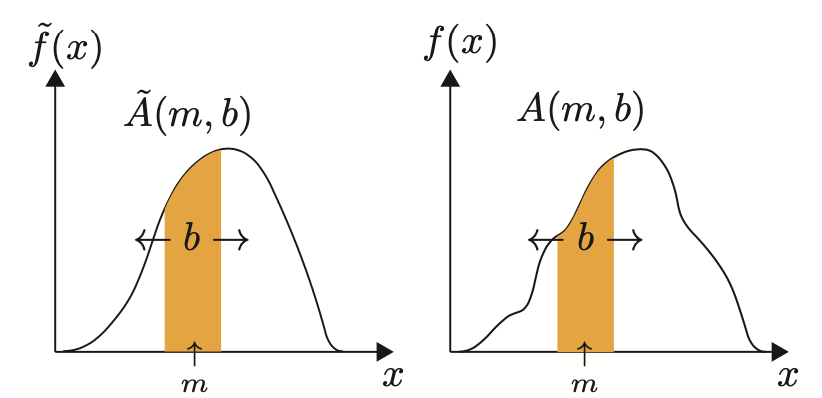
Compare $\tilde{A}(m, b)$ and $A(m,b), \forall m, b$
Symmetric, unique, but redundant…
Multivariate case (2D)
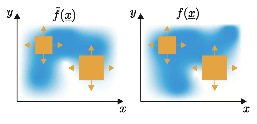
Different kernels possible
- Rectangular kernels
- Gaussian kernels
- Anisotropic vs. isotropic kernels
- Separable vs. inseparable kernels
Cumulative Transformation of Densities
Given
- Random vector $\underline{x} \in \mathbb{R}^N$
- Probability density function $f(\underline{x}): \mathbb{R}^N \to \mathbb{R}_+$
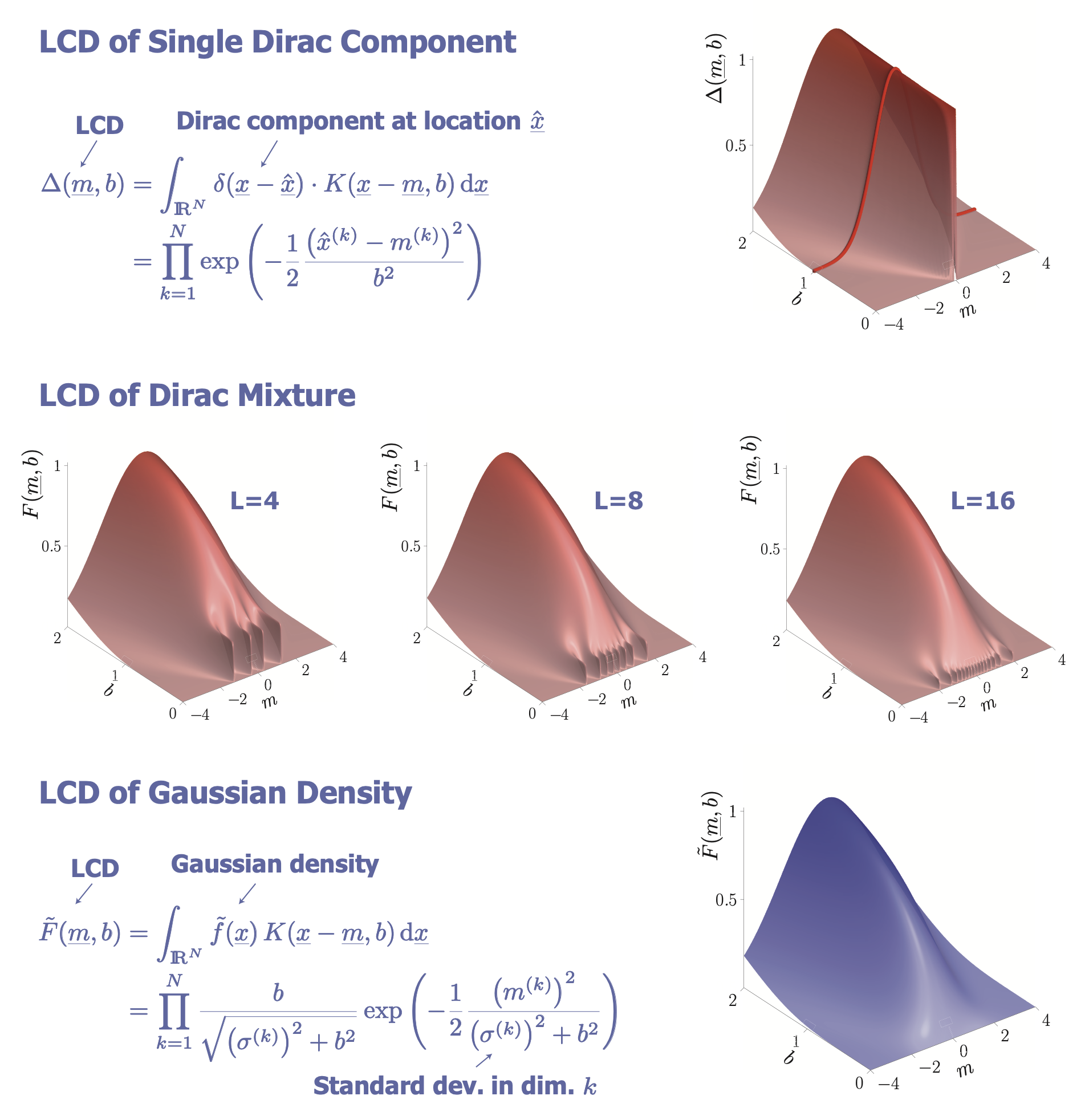
Localized Cumulative Distribution (LCD):
$$ F(\underline{m}, b)=\int_{\mathbb{R}^{N}} f(\underline{x}) K(\underline{x}-\underline{m}, b) \mathrm{d} \underline{x} $$- $K(\cdot, \cdot)$: Kernel
- $\underline{m}$: Kernel location
- $\underline{b}$: Kernel width
Specific kernel employed:
$$ K(\underline{x}-\underline{m}, b)=\prod_{k=1}^{N} \exp \left(-\frac{1}{2} \frac{\left(x_{k}-m_{k}\right)^{2}}{b^{2}}\right) $$- Separable (i.e. in form of product)
- isotropic (i.e. same in each direction)
- Gaussian
Properties of LCD:
- Symmetric
- Unique
- Multivariate
Examples
LCD (Rectangular Kernel)
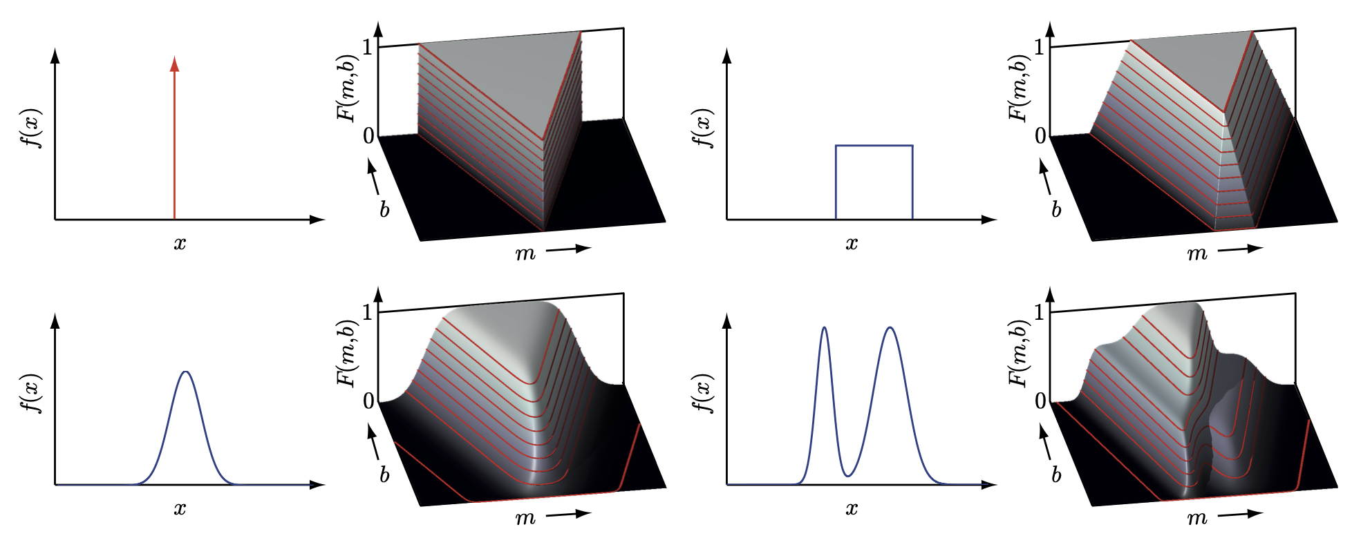
LCD (Gaussian Kernel)
Generalized Cramér–von Mises Distance (GCvD)
Given:
- LCD of given continuous density $\tilde{F}(\underline{m}, b)$
- LCD of Dirac mixture $F(\underline{m}, b)$
Definition:
$$ D=\int_{\mathbb{R}_{+}} w(b) \int_{\mathbb{R}^{N}}(\tilde{F}(\underline{m}, b)-F(\underline{m}, b))^{2} \mathrm{~d} \underline{m} \mathrm{~d} b $$Minimization of GCvD:
- For many Dirac components → high-dimensional optimization problem
- Gradient available, Hessian more difficult
- Use Quasi-Newton method: L-BFGS
Projected Cumulative Distributions (PCD)
Options for Reduction to Univariate Case
Reapproximation methods for univariate case readily available. How can we use univariate methods in multivariate case?
Solution
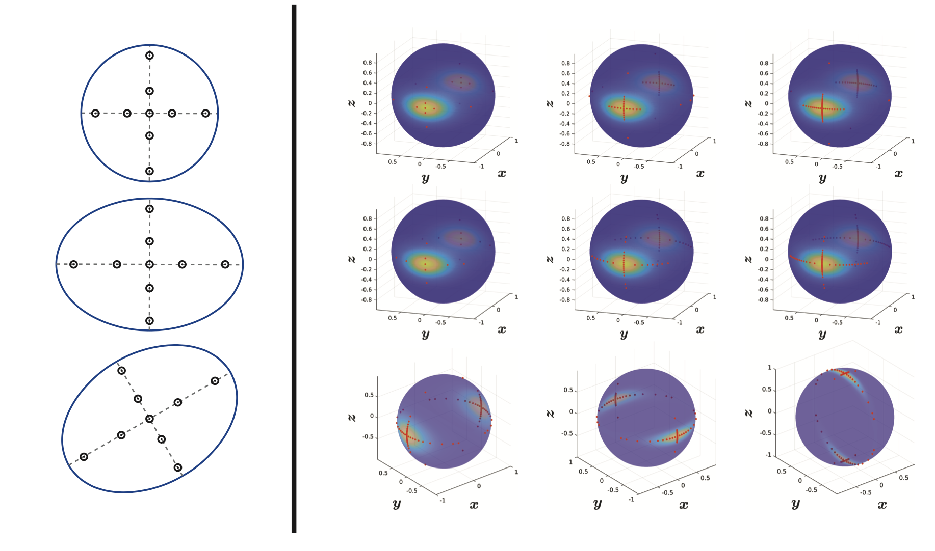
Approximation on principal axis of PDF
- Limited to densities where principal axis can be defined
- Examples: Gaussian PDF, Bingham PDF on sphere
- Does not cover the entire density 🤪
Cartesian product of 1D approximation 👎
- Curse of dimensionality (as very similar to grid)
- Only for product densities (or rotations thereof)
- Inefficient coverage
Representing PDFs by all one-dimensional projections (a.k.a Radon transform) 👍
Represent the two densities $\tilde{f}(\underline{x})$ and $f(\underline{x})$ by infinite set of one-dimensional projections
Projections onto all unit vectors $\underline{u} \in \mathbb{S}^{N-1}$
We obtain sets of projections $\tilde{f}(r \mid \underline{u})$ and $f(r \mid u)$ ($r$: the density along the unit vector)
These are the Radon transforms of $\tilde{f}(\underline{x})$ and $f(\underline{x})$
We compare the sets of projections $\tilde{f}(r \mid \underline{u})$ and $f(r \mid u)$ for every $\underline{u} \in \mathbb{S}^{N-1}$
For comparison, we use the univariate cumulative distribution functions $\tilde{F}(r \mid \underline{u})$ and $F(r \mid u)$
These are unique, well defined, and easy to calculate 👏
Resulting distance measures
$$ D_{1}(\underline{u})=D(\tilde{f}(r \mid \underline{u}), f(r \mid \underline{u})) $$depend on the projection vector $\underline{u}$
We integrate these one-dimensional distance measures $D_1(\underline{u})$ over all unit vectors $\underline{u} \in \mathbb{S}^{N-1}$
- This gives multivariate distance measure $D(\tilde{f}(\underline{x}), f(\underline{x}))$
- Typically a discretized subset of $\underline{u} \in \mathbb{S}^{N-1}$ is used
- Distance measure minimized via univariate Newton updates
Radon Transform
Represent general $N$-dimensional probability density functions via the set of all one-dimensional projections
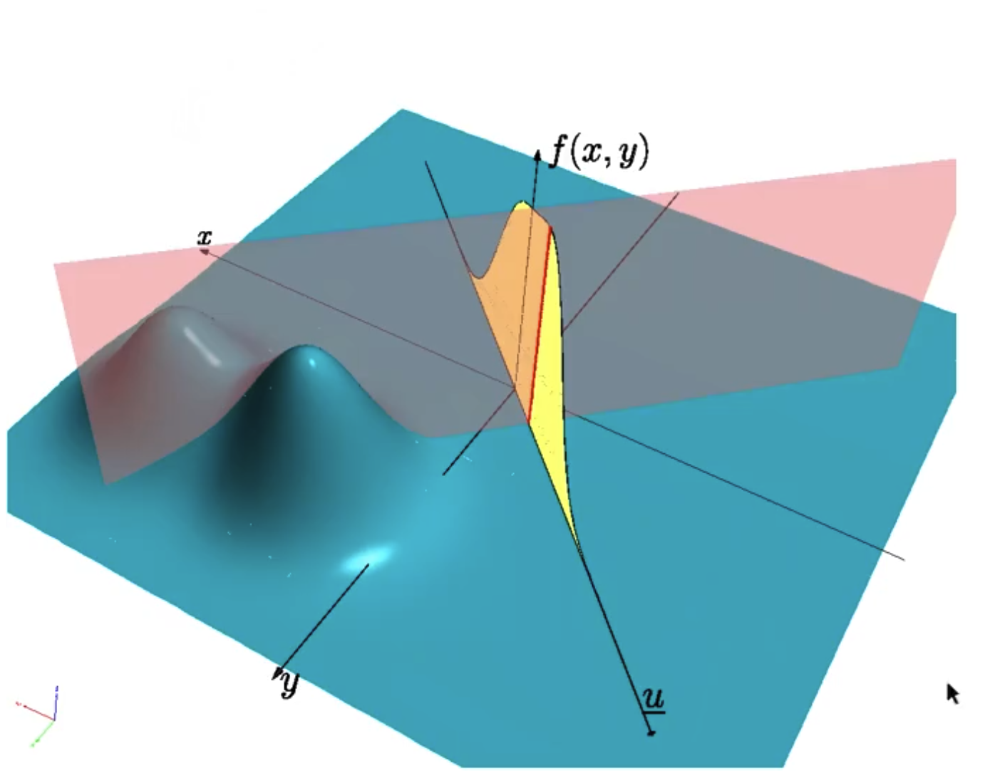
Linear projection of random vector $\underline{\boldsymbol{x}} \in \mathbb{R}^{N}$ to scalar random variable $\boldsymbol{r} \in \mathbb{R}$ onto line described by unit vector $\underline{u} \in \mathbb{S}^{N-1}$
$$ \boldsymbol{r} = \underline{u}^\top \underline{\boldsymbol{x}} $$Given probability density function $f(\underline{x})$ of random vector $\underline{\boldsymbol{x}}$, density $f_r(r \mid \underline{u})$ of $\boldsymbol{r}$ is given by
$$ f_{r}(r \mid \underline{u})=\int_{\mathbb{R}^{N}} f(\underline{t}) \delta\left(r-\underline{u}^{\top} \underline{t}\right) \mathrm{d} \underline{t} $$$f_r(r \mid \underline{u})$ is Radon transform of $f(\underline{x})$ for all $\underline{u} \in \mathbb{S}^{N-1}$
Visualization:
$u$ is the unit vector.
We project the density on $u$ and we get the projection (yellow area).
Then if we cut through the projection, it gives us the red line.

Dirac Mixture Densities
$$ f(\underline{x} \mid \hat{\mathbf{X}})=\sum_{i=1}^{L} w_{i} \delta\left(\underline{x}-\underline{\hat{x}}_{i}\right) $$with
$$ \hat{\mathbf{X}}=\left[\underline{\hat{x}}_{1}, \underline{\hat{x}}_{2}, \ldots, \underline{\hat{x}}_{L}\right] $$Radon transform is given by
$$ f_{r}(r \mid \underline{\hat{r}}, \underline{u})=\sum_{i=1}^{L} w_{i} \delta\left(\underline{u}^{\top} \underline{x} - \underline{u}^{\top} \underline{\hat{x}}_{i}\right)=\sum_{i=1}^{L} w_{i} \delta\left(r-\hat{r}_{i}(\underline{u})\right) $$- $\hat{r}_{i}(\underline{u})=\underline{u}^{\top} \underline{x}_{i}, i=1, \ldots, L$ are the projected Dirac locations
Collect projected Dirac locations $\hat{r}_{i}(\underline{u})$ in vector
$$ \underline{\hat{r}}=\left[\hat{r}_{1}(\underline{u}), \hat{r}_{2}(\underline{u}), \ldots, \hat{r}_{L}(\underline{u})\right]^{\top} $$Gaussian Densities
For Gaussian Density $f (\underline{x}) $with mean vector $\underline{\hat{x}}$ and covariance matrix $\mathbf{C}_x$, density $f_r(r \mid \underline{u})$ resulting from the projection is also Gaussian
Its mean $\hat{r}(\underline{u})$ can simply be calculated by taking the expected value
$$ \hat{r}(\underline{u})=\mathrm{E}\{\boldsymbol{r}(\underline{u})\}=\mathrm{E}\left\{\underline{u}^{\top} \underline{\boldsymbol{x}}\right\}=\underline{u}^{\top} \underline{\hat{x}} $$Its standard deviation $\sigma_r(\underline{u})$ is given by
$$ \sigma_{r}^{2}(\underline{u})=\mathrm{E}\left\{(\boldsymbol{r}(\underline{u})-\hat{r}(\underline{u}))^{2}\right\}=\mathrm{E}\left\{\left(\underline{u}^{\top} \boldsymbol{x}-\underline{u}^{\top} \underline{\hat{x}}\right)^{2}\right\}=\mathrm{E}\left\{\underline{u}^{\top}(\boldsymbol{x}-\underline{\hat{x}})(\boldsymbol{x}-\underline{\hat{x}})^{\top} \underline{u}\right\}=\underline{u}^{\top} \mathbf{C}_{x} \underline{u} $$
Gaussian Mixture Densities
For $N$-dimensional Gaussian mixture densities $f(\underline{x})$ of the form
$$ f(\underline{x})=\sum_{i=1}^{M} w_{i} \frac{1}{\sqrt{(2 \pi)^{N}\left|\mathbf{C}_{x, i}\right|}} \exp \left(-\frac{1}{2}\left(\underline{x}-\underline{\hat{x}}_{i}\right)^{\top} \mathbf{C}_{x, i}^{-1}\left(\underline{x}-\underline{\hat{x}}_{i}\right)\right) $$the density $f_r(r, \underline{u})$ is also a Gaussian mixture
Due to the linearity of the projection operator, it is given by
$$ f_{r}(r \mid \underline{u})=\sum_{i=1}^{M} w_{i} \frac{1}{\sqrt{2 \pi} \sigma_{r, i}(\underline{u})} \exp \left(-\frac{1}{2} \frac{\left(r-\hat{r}_{i}(\underline{u})\right)^{2}}{\sigma_{r, i}^{2}(\underline{u})}\right) $$with
$$ \hat{r}_{i}(\underline{u})=\underline{u}^{\top} \underline{\hat{x}}_{i} $$and
$$ \sigma_{r, i}(\underline{u})=\sqrt{\underline{u}^{\top} \mathbf{C}_{x, i} \underline{u}} $$
Multivariate Cramér-von Mises Distance
Multivariate distance measure between two continuous and/or discrete probability density functions
One-dimensional Projections via Radon Transform
Given density $\tilde{f}(\underline{x})$ and its approximation $f(\underline{x})$, represented by their Radon transforms $\tilde{f}(r \mid \underline{u})$ (i.e. by their 1D projections onto unit vectors $\underline{u} \in \mathbb{S}^{N-1}$)
One-dimensional Cumulative Distributions
Based on Radon transform $\tilde{f}(r \mid \underline{u})$, calculate one-dimensional cumulative distributions of the projected densities as
$$ \tilde{F}(r \mid \underline{u})=\int_{\infty}^{r} \tilde{f}(t, \underline{u}) \mathrm{d} t $$and similarly for $F(r \mid \underline{u})$
Example: For Dirac mixture approximation, cumulative distribution function of its Radon transform is given by
$$ F(r \mid \underline{\hat{r}}, \underline{u})=\sum_{i=1}^{L} w_{i} \mathrm{H}\left(r-\hat{r}_{i}(\underline{u})\right) $$
One-dimensional Distance
For comparing the one-dimensional projections, we compare their cumulative distributions $\tilde{F}(r \mid \underline{u})$ and $F(r \mid \underline{\hat{r}}, \underline{u})$ for all $\underline{u} \in \mathbb{S}^{N-1}$
As distance measure use integral squared distance
$$ D_{1}(\underline{\hat{r}}, \underline{u})=\int_{\mathbb{R}}[\tilde{F}(r \mid \underline{u})-F(r \mid \underline{\hat{r}}, \underline{u})]^{2} \mathrm{~d} r $$Gives distance between the projected densities in the direction of the unit vector $\underline{u}$ for all $\underline{u}$
One-dimensional Newton Step
- Newton step can now be written as
with
$$ \begin{aligned} \underline{G}(\underline{\hat{r}}, \underline{u})&=\left[\frac{\partial D_{1}(\underline{\hat{r}}, \underline{u})}{\partial \hat{r}_{1}}, \frac{\partial D_{1}(\underline{\hat{r}}, \underline{u})}{\partial \hat{r}_{2}}, \ldots, \frac{\partial D_{1}(\underline{\hat{r}}, \underline{u})}{\partial \hat{r}_{L}}\right]^{\top} \\ \frac{\partial D_{1}(\underline{\hat{r}}, \underline{u})}{\partial \hat{r}_{i}}&=2 w_{i}\left[\tilde{F}\left(\hat{r}_{i} \mid \underline{u}\right)-F\left(\hat{r}_{i} \mid \underline{u}\right)\right] \end{aligned} $$Hessian $\mathbf{H}(\underline{r}, \underline{u})$ is given by
$$ \mathbf{H}(\underline{\hat{r}}, \underline{u})=2 \operatorname{diag}\left(\left[w_{1} \tilde{f}\left(\hat{r}_{1} \mid \underline{u}\right), w_{2} \tilde{f}\left(\hat{r}_{2} \mid \underline{u}\right), \ldots, w_{L} \tilde{f}\left(\hat{r}_{L} \mid \underline{u}\right)\right]\right) $$$\Rightarrow$ Resulting Newton step
$$ \Delta \underline{\hat{r}}(\underline{\hat{r}}, \underline{u})=-\left[\frac{\tilde{F}\left(\hat{r}_{1} \mid \underline{u}\right)-F\left(\hat{r}_{1} \mid \underline{\hat{r}}, \underline{u}\right)}{\tilde{f}\left(\hat{r}_{1} \mid \underline{u}\right)}, \ldots, \frac{\tilde{F}\left(\hat{r}_{L} \mid \underline{u}\right)-F\left(\hat{r}_{L} \mid \underline{\hat{r}}, \underline{u}\right)}{\tilde{f}\left(\hat{r}_{L} \mid \underline{u}\right)}\right]^{\top} $$
Backprojection to $N$-dimensional space
For specific projection vector $\underline{u}$: Newton update $\Delta \underline{\hat{r}}(\underline{\hat{r}}, \underline{u})$
Backprojection into original $N$-dimensional space: Update can be used to modify original Dirac locations in direction along the vector $\underline{u}$
For every location vector $\underline{\hat{x}}_i$ we obtain
$$ \Delta \underline{\hat{x}}_{i}(\underline{u})=\Delta \underline{\hat{r}}(\underline{\hat{r}}, \underline{u}) \cdot \underline{u} $$
Assemble Multivariate Distance
Individual 1D distances $D_1(\underline{r}, \underline{u})$ can be assembled to form multivariate distance measure
Performed by integrating over all 1D distances depending on unit vector $\underline{u}$
$$ D_{N}(\hat{\mathbf{X}})=\int_{\mathbb{S}^{N-1}} D_{1}(\underline{\hat{r}}, \underline{u}) \mathrm{d} \underline{u} $$Plugging in $D_1(\underline{r}, \underline{u})$:
$$ D_{N}(\hat{\mathbf{X}})=\int_{\mathbb{S}^{N-1}} \int_{\mathbb{R}}[\tilde{F}(r \mid \underline{u})-F(r \mid \underline{\hat{r}}, \underline{u})]^{2} \mathrm{~d} r \mathrm{~d} \underline{u} \quad \text { with } r=\underline{u}^{\top} \cdot \underline{x} $$
Perform Full Newton Update
Full Newton update by integrating over all partial updates along projection vectors $\underline{u}$
$$ \Delta \underline{\hat{x}}_{i}=\int_{\mathbb{S}^{N-1}} \Delta \underline{\hat{x}}_{i}(\underline{u}) \mathrm{d} \underline{u} $$
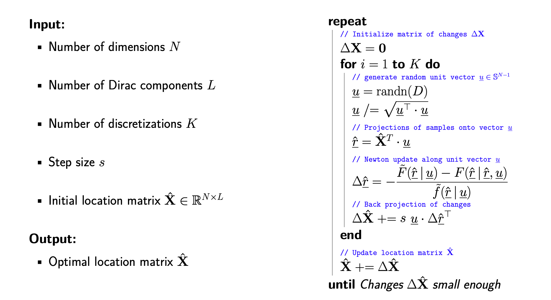
Discretization of Space of Unit Vectors
In practice, Space $\mathbb{S}^{N-1}$ containing unit vectors $\underline{u}$ has to be discretized
Two options are available for performing the discretization:
- Deterministic discretization, e.g., by calculating a grid
- Random discretization by drawing uniform samples from the hypersphere
For both cases: Consider $K$ samples $\underline{u}_k$
Integration reduces to summation
$$ \Delta \underline{\hat{x}}_{i} \approx \frac{1}{K} \sum_{k=1}^{K} \Delta \underline{\hat{x}}_{i}\left(\underline{\hat{u}}_{k}\right) \quad \text { for } i=1,2, \ldots, L $$Stopping criterion
Given initial locations for the location of the Dirac components
Full Newton updates are performed until the maximum change over all location vectors
$$ \max _{i}\left|\Delta \underline{\hat{x}}_{i}\right| $$falls below a given threshold
Complete Algorithm (Randomized Variant)