Ensemble Kalmanfilter (EnKF)
Motivation
Prädiktionsschritt von Nichtlineares Kalmanfilter (NLKF) $\rightarrow$ speziell Variante sample-basiert
Durch Re-approximation mit Gaußdichte $\rightarrow$ Zusatzinformation verloren
Wenn keine Messungen vorliegen und mehrere Prädiktionsschritte nacheinander $\rightarrow$ Man kann temporär Approximation fortlassen
Filterschritt von NLKF
$$ \begin{array}{l} \underline{\hat{x}}_{e}=\underline{\hat{x}}_{p}+\mathbf{C}_{x y} \mathbf{C}_{y y}^{-1}(\underline{\hat{y}}-E\{\underline{h}(\underline{x})\}) \\ \mathbf{C}_{e}=\mathbf{C}_{p}-\mathbf{C}_{x y} \mathbf{C}_{y y}^{-1} \mathbf{C}_{y x} \end{array} $$wobei
$$ \begin{array}{ll} \mathbf{C}_{x x}=\mathbf{C}_{p} \in \mathbb{R}^{N \times N}\quad &\mathbf{C}_{x y} \in \mathbb{R}^{N \times M} \\ \mathbf{C}_{y x} \in \mathbb{R}^{M \times N}\quad &\mathbf{C}_{yy} \in \mathbb{R}^{M \times M} \end{array} $$Unabhängig von gewähltes Form der Momenteberechnung $\rightarrow$ Hoher Aufwand für Berechnung und Speichern der Kovairanzmatrizen 🤪
Idee
Beibehaltung der Samples nach Prädiktionsschritt $\rightarrow$ Keine Re-approximation durch Gauß
Damit bleibt Forminformation erhalten und Unsicherheit wird in samples gespeichert.
Speicherkomplexität
Kalmanfilter (KF)
- Erwartungswert; $N$
- Kovarianzmatrix $\frac{N(N+1)}{2}$
$\Rightarrow$ Insgesamt $\frac{N^2 + 3N}{2}$
EnKF
- Ein sample: $N$
- $L$ samples: $L \cdot N$ (z.B mit sampling auf der Hauptachse gilt $L = 2N \rightarrow 2N^2$)
Aber: spart Aufwand bei Berechnung der Kovarianzmatrix
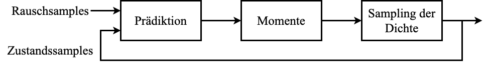
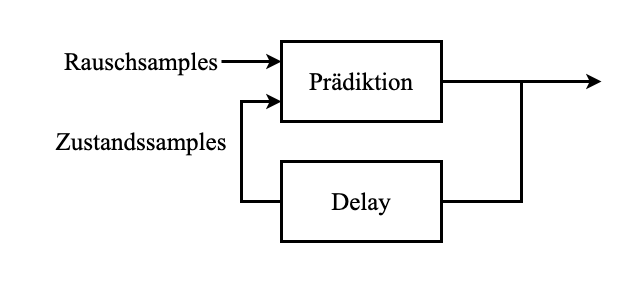
🎯 Ziel: Rekursive Berechnung des Prädiktionsschritts
Herausforderungen
Gegeben
$L$ Samples $\underline{x}_{k, i}, i = 1, \dots, L$
Systemabbildung
$$ \underline{x}_{k+1} = \underline{a}_k(\underline{x}_k, \underline{w}_k) $$
Gesucht: $L^\prime$ Samples $\underline{x}_{k, i+1}, i = 1, \dots, L^\prime$
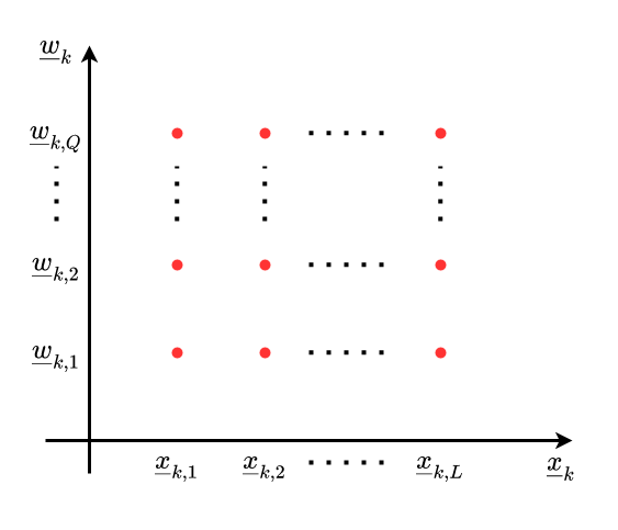
Wir benötigen Samples für $\underline{w}_k$: $\underline{w}_{k, j}, j = 1, \dots, Q$
‼️ Problem: Abbildung der Kombination aller Samples $\Rightarrow$ Kartesisches Produkt!!! $\Rightarrow$ Anzahl der Samples steigt bei rekursiver Prädiktion exponentiell !!!
Lösungsidee: Begrenzung der Abtastwerte
- Ziel: Einstellbare Anzahl an Samples $\rightarrow$ um Komplexität zu folgen
- Einfacher Fall: Konstante Anzahl Samples über Zeit
Anzatz 1: Über Reduktion
Prior
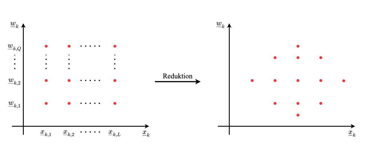
Posterior (also Reduktion von $\underline{x}_{k+1, i}$ )
- braucht $L \cdot Q$ Abbildungen
- Ergebnis aber oft besser
Ansatz 2: Anzahl von Parren mit Latin Hypercube Sampleing (LHS)
Jede Zeile und Spalte darf NUR ein Element erhalten
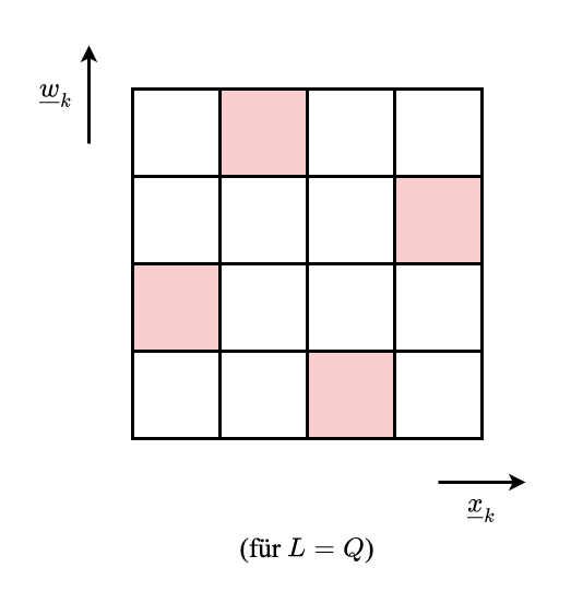
Optimale Wahl schwierig
- Diskretes Gütemaß ist i.d.R. zimliche kompliziert
Triviale praktische Umsetzung: Ziehe (Konstante) Samples aus $\underline{w}_k$ für jedes $\underline{x}_{k, i}$ (aber schlecht für wenige Samples)
Anordnung
$$ \mathcal{X}_{k}=[\underbrace{\underline{x}_{k, 1}}_{\mathbb{R}^N}, \underline{x}_{k, 2}, \ldots, \underline{x}_{k, L}] \in \mathbb{R}^{N \times L}, \quad \mathcal{W}_{k}=\left[\underline{w}_{k, 1}, \underline{w}_{k, 2}, \ldots, \underline{w}_{k, L}\right] \in \mathbb{R}^{N \times L} $$Jede $\underline{x}_{k, i}$ und $\underline{w}_{k, j}$ ist ein Vektor.
$\underline{a}_k$ überladen:
$$ \mathcal{X}_{k+1} = \underline{a}_k(\mathcal{X}_{k}, \mathcal{W}_{k}) $$
Filterschritt
🎯 Ziel
- Durchführung der Filterschritt NUR mit Samples
- Direkte Überführung der prioren Samples in posteriore Samples
- Vermeidung der Verwendung der Update-Formeln für Kovarianzmatrix
- Reine Representation der Unsicherheiten durch Samples
Lineare Messungabbildung
$$ \underline{y}=\mathbf{H} \cdot \underline{x}+\underline{v} $$Für gegebene Messung $\hat{y}$:
$$ \underbrace{\underline{\hat{y}}-\underline{v}}_{=:\hat{\mathcal{Y}}}=\mathbf{H} \cdot \underline{x} $$Mess-sampleset:
$$ \hat{\mathcal{Y}}=\underline{\hat{y}} \cdot \underline{\mathbb{1}}^{\top}-\mathcal{V} \qquad \mathcal{V}=\left[\underline{v}_{1}, \underline{v}_{2}, \ldots, \underline{v}_{L}\right] $$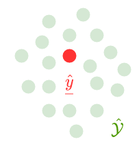
Damit ist Update des Zustands in “combination form”
$$ \mathcal{X}_{e}=(\mathbf{I}-\mathbf{K} \mathbf{H}) \mathcal{X}_{p}+\mathbf{K} \mathcal{\hat{Y}} $$$\mathcal{X}$ und $\mathcal{Y}$ sind Matrizen
wäre begrenzt auf additives Rauschen, aber funktioniert direkt für nichtlineare Messabbildung $\underline{y}=\underline{h}(\underline{x}, \underline{v})$.
Alternative Herleitung
Prädizierte Mess-samples basierend auf prioren Samples und Rauschen-samples:
$$ \mathcal{Y} = \mathbf{H} \cdot \mathcal{X}_p + \mathcal{V} $$Update des Zustands in “feedback form”
$$ \begin{aligned} \mathcal{X}_e &= \mathcal{X}_p + \mathbf{K}(\underbrace{\underline{\hat{y}} \cdot \underline{\mathbf{1}}^\top}_{\text{gemessen}} - \underbrace{\mathcal{Y}}_{\text{Prädiktion}}) \\\\ &= \mathcal{X}_e + \mathbf{K}(\underline{\hat{y}} \cdot \underline{\mathbf{1}}^\top - \mathbb{H} \mathcal{X}_p - \mathcal{V})\\\\ &= (\mathbb{I} - \mathbf{K}\mathbf{H})\mathcal{X}_p + \mathbf{K}(\underbrace{\underline{\hat{y}} \cdot \underline{\mathbf{1}}^\top - \mathcal{V}}_{=\hat{\mathcal{Y}}}) \end{aligned} $$