Pattern Recognition

Why pattern recognition and what is it?

What is machine learning?

• Motivation: Some problems are very hard to solve by writing a computer program by hand
• Learn common patterns based on either

  • a priori knowledge or

  • on statistical information

    • Important for the adaptability to different tasks/domains
    • Try to mimic human learning / better understand human learning
• Machine learning is concerned with developing generic algorithms, that are able to solve problems by learning from example data

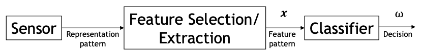
Classifiers

• Given an input pattern $\mathbf{x}$, assign in to a class $\omega\_i$

  • Example: Given an image, assign label “face” or “non-face”
  • $\mathbf{x}$: can be an image, a video, or (more commonly) any feature vector that can be extracted from them
  • $\omega\_i$: desired (discrete) class label
    • If “class label” is real number or vector –> Regression task

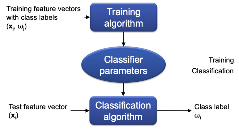
• ML: Use example patterns with given class labels to automatically learn

  

• Example

  

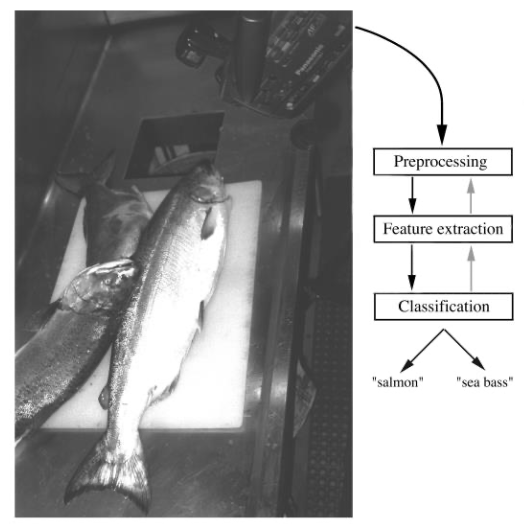
• Classification process

  

Bayes Classification

• Given a feature vector $\mathbf{x}$, want to know which class $\omega\_i$ is most likely

• Use Bayes’ rule: Decide for the class $\omega\_i$ with maximum posterior probability

  

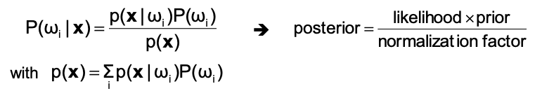
• 🔴 Problem: $p(x|\omega\_i)$ (and to a lesser degree $P(\omega\_i)$) is usually unknown and often hard to estimate from data

• Priors describe what we know about the classes before observing anything

  • Can be used to model prior knowledge

  • Sometimes easy to estimate (counting)

• Example

  

Gaussian Mixture Models

Gaussian classification

• Assumption:

  $$\mathrm{p}\left(\mathbf{x} | \omega_{\mathrm{i}}\right) \sim \mathrm{N}(\boldsymbol{\mu}, \mathbf{\Sigma})= \frac{1}{(2 \pi)^{d / 2}|\Sigma|^{1 / 2}} \exp \left[-\frac{1}{2}(\mathbf{x}-\boldsymbol{\mu})^{\top} \boldsymbol{\Sigma}^{-1}(\mathbf{x}-\boldsymbol{\mu})\right]$$
  • 👆 This makes estimation easier
    • Only $\boldsymbol{\mu}, \mathbf{\Sigma}$ need to be estimated
    • To reduce parameters, the covariance matrix can be restricted

      • Diagonal matrix –> Dimensions uncorrelated

      • Multiple of unit matrix –> Dimensions uncorrelated with same variance

• 🔴 Problem: if the assumption(s) do not hold, the model does not represent reality well 😢

• Estimation of $\boldsymbol{\mu}, \mathbf{\Sigma}$ with Maximum (Log-)Likelihood

  • Use parameters, that best explain the data (highest likelihood):

    $$\begin{aligned} \operatorname{Lik}(\boldsymbol{\mu}, \mathbf{\Sigma}) &= p(\text{data}|\boldsymbol{\mu}, \mathbf{\Sigma}) \\\\ &= p(\mathbf{x}\_0, \mathbf{x}\_1, \dots, \mathbf{x}\_n|\boldsymbol{\mu}, \mathbf{\Sigma}) \\\\ &= p\left(\mathbf{x}\_{0} | \boldsymbol{\mu}, \mathbf{\Sigma}\right) \cdot p\left(\mathbf{x}\_{1} | \boldsymbol{\mu}, \mathbf{\Sigma}\right) \cdot \ldots \cdot p\left(\mathbf{x}\_{\mathrm{n}} | \boldsymbol{\mu}, \mathbf{\Sigma}\right) \end{aligned}$$ $$\operatorname{LogLik}(\boldsymbol{\mu}, \mathbf{\Sigma}) = \log(\operatorname{Lik}(\boldsymbol{\mu}, \mathbf{\Sigma})) = \sum\_{i=0}^n \log(\mathbf{x}\_i | \boldsymbol{\mu}, \mathbf{\Sigma})$$

    –> Maimize $\log(\operatorname{Lik}(\boldsymbol{\mu}, \mathbf{\Sigma}))$ over $\boldsymbol{\mu}, \mathbf{\Sigma}$

Gaussian Mixture Models (GMMs)

• Approximate true density function using a weighted sum of several Gaussians

  $$\mathrm{p}(\mathbf{x})=\sum\_{i} \mathrm{w}\_{i} \frac{1}{(2 \pi)^{\mathrm{d}/2}|\mathbf{\Sigma}|^{1 / 2}} \exp \left[-\frac{1}{2}(\mathbf{x}-\mathbf{\mu})^{\top} \boldsymbol{\Sigma}^{-1}(\mathbf{x}-\boldsymbol{\mu})\right] \qquad \text{with} \sum\_i w\_i = 1$$

• Any density can be approximated this way with arbitrary precision

  • But might need many Gaussians
  • Difficult to estimate many parameters

• Use Expectation Maximization (EM) Algorithm to estimate parameters of the Gaussians as well as the weights

  1. Initialize parameters of GMM randomly

  2. Repeat until convergence

     • Expectation (E) step:

       Compute the probability $p\_{ij}$ that data point $i$ belongs to Gaussian $j$

       • Take the value of each Gaussian at point $i$ and normalize so they sum up to one

     • Maximization (M) step:

       Compute new GMM parameters using soft assignments $p\_{ij}$

       • Maximum Likelihood with data weighted according to $p\_{ij}$

Linear Discriminant Functions

• Separate two classes $\omega\_1, \omega\_2$ with a linear hyperplane

  $$y(x)=w^{T} x+w_{0}$$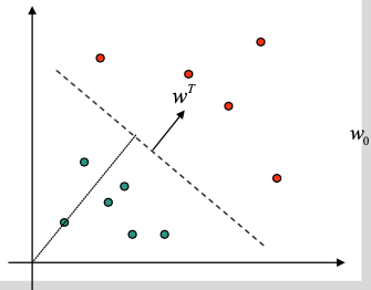

  

  • Decide $\omega\_1$ if $y(x) > 0$ else $\omega\_2$
  • $w^T$: normal vector of the hyperplane

• Example:

  • Perceptron (see: Perceptron)
  • Linear SVM

Support Vector Machines

See: SVM

Linear SVMs

• If the input space is already high-dimensional, linear SVMs can often perform well too
• 👍 Advantages:
  • Speed: Only one scalar product for classification
  • Memory: Only one vector w needs to be stored
  • Training: Training is much faster
  • Model selection: Only one parameter to optimize

K-nearest Neighbours

• 💡 Look at the $k$ closest training samples and assign the most frequent label among them

• Model consists of all training samples

  • Pro: No information is lost

  • Con: A lot of data to manage

• Naïve implementation: compute distance to each training sample every time

  • Distance metric is needed (Important design parameter!)
    • $L\_1$, $L\_2$, $L\_{\infty}$, Mahalanobis, … or
    • Problem-specific distances

• kNN often good classifier, but:

  • Needs enough data
  • Scalability issues

Clustering

• New problem setting
  • Only data points are given, NO class labels
  • Find structures in given data
• Generally no single correct solution possible

K-means

• Algorithm

  1. Randomly initialize k cluster centers

  2. Repeat until convergence:

     • Assign all data points to closest cluster center

     • Compute new cluster center as mean of assigned data points

• 👍 Pros: Simple and efficient

• 👎 Cons:

  • $k$ needs to be known in advance
  • Results depend on initialization
  • Does not work well for clusters that are not hyperspherical (round) or clusters that overlap

• Very similar to the EM algorithm

  • Uses hard assignments instead of probabilistic assignments (EM)

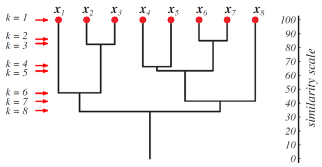
Agglomerative Hierarchical Clustering

• Algorithm

  1. Start with one cluster for each data point

  2. Repeat

     • Merge two closest clusters

• Several possibilities to measure cluster distance

  • Min: minimal distance between elements

  • Max: maximal distance between elements

  • Avg: average distance between elements

  • Mean: distance between cluster means

• Result is a tree called a dendrogram

• Example:

  

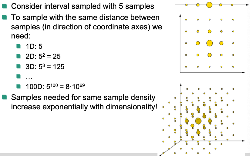
Curse of dimensionality

• In computer vision, the extracted feature vectors are often high-dimensional

• Many intuitions about linear algebra are no longer valid in high-dimensional spaces 🤪

  • Classifiers often work better in low-dimensional spaces

• These problems are called “curse of dimensionality" 👿

Example

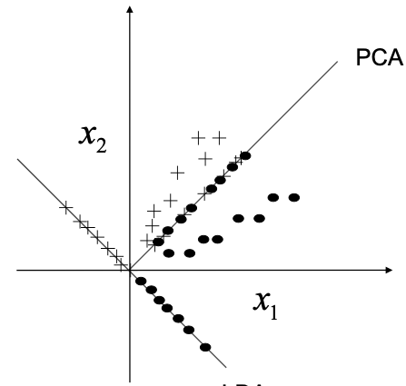
Dimensionality reduction

• PCA: Leave out dimensions and minimize error made

  

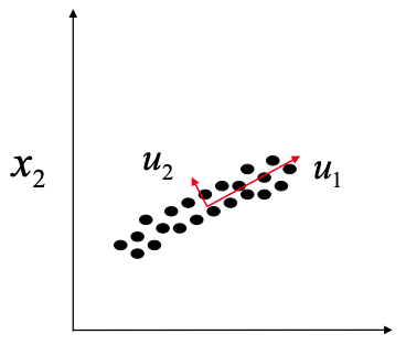
• LDA: Maximize class separability