Facial Feature Detection

Introduction

What are facial features?

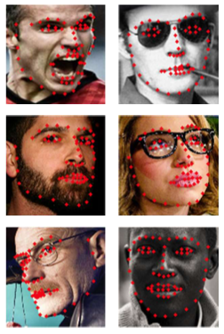
Facial features are referred to as salient parts of a face region which carry meaningful information.

• E.g. eye, eyeblow, nose, mouth
• A.k.a facial landmarks

What is facial feature detection?

Facial feature detection is defined as methods of locating the specific areas of a face.

Applications of facial feature detection

• Face recognition
• Model-based head pose estimation
• Eye gaze tracking
• Facial expression recognition
• Age modeling

Problems in facial feature detection

• Identity variations

  Each person has unique facial part

• Expression variations

  Some facial features change their state (e.g. eye blinks).

• Head rotations

  If a head orientation changes, the visual appearance also changes.

• Scale variations

  Changes in resolution and distance to the camera affect appearance.

• Lighting conditions

  Light has non-linear effects on the pixel values of a image.

• Occlusions

  Hair or glasses might hide facial features.

Older approaches (from face detection)

• Integral projections + geometric constraints
• Haar-Filter Cascades
• PCA-based methods (Modular Eigenspace)
• Morphable 3D Model

Statistical appearance models

• 💡 Idea: make use of prior-knowledge, i.e. models, to reduce the complexity of the task
• Needs to be able to deal with variability $\rightarrow$ deformable models
• Use statistical models of shape and texture to find facial landmark points
• Good models should
  • Capture the various characteristics of the object to be detected
  • Be a compact representation in order to avoid heavy calculation
  • Be robust against noise

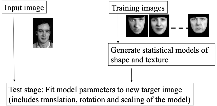
Basic idea

1. Training stage: construction of models
2. Test stage: Search the region of interest (ROI)

Appearance models

• Represent both texture and shape

• Statistical model learned from training data

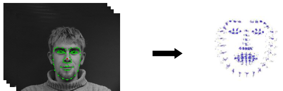
• Modeling shape variability

  • Landmark points
  $$x=\left[x\_{1}, y\_{1}, x\_{2}, y\_{2}, \ldots, x\_{n}, y\_{n}\right]^{T}$$

  • Model

    $$x \approx \bar{x}+P\_{s} b\_{s}$$
    • $\bar{x}$: Mean vector
    • $P\_s$: Eigenvectors of covariance matrix
    • $b\_s = P\_s^T(x - \bar{x})$

• Modeling intensity variability:

  • Gray values

    $$h=\left[g\_{1}, g\_{2}, \ldots, g\_{k}\right]^{T}$$

  • Model

    $$h \approx \bar{h} + P\_ib\_i$$
    • $\bar{h}$: Mean vector
    • $P\_s$: Eigenvectors of covariance matrix
    • $b\_i = P\_i^T(h - \bar{h})$

Training of appearance models

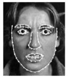
1. Construct a shape model with Principal component analysis (PCA)

A shape is represented with manually labeled points.

The shape model approximates the shape of an object.

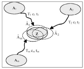
Procrustes Analysis

Align the shapes all together to remove translation, rotation and scaling

PCA

The positions of labeled points are

• $\bar{x}$: Mean shape
• $P\_s$: Orthogonal modes of variation obtained by PCA
• $b\_s$: Shape parameters in the projected space

The shapes are represented with fewer parameters ($\operatorname{Dim}(x) > \operatorname{Dim}(b\_s)$)

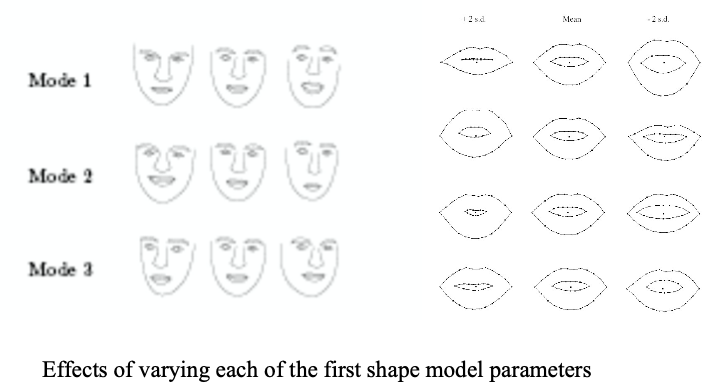
Generating plausible shapes:

2. Construct a texture model which represents grey-scale (or color) values at each point

Warp the image so that the labeled points fit on the mean shape

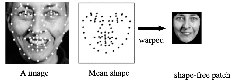
Then normalize the intensity on the shape-free patch.

Texture warping

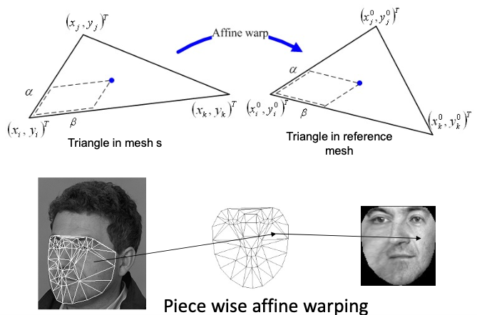
Texture model

The pixel values on the shape-free patch

• $\bar{g}$ : Mean of normalized pixel values
• $P\_g$ : Orthogonal modes of variation obtained by PCA
• $b\_g$: Texture parameters in the projected space

The pixel values (appearance) are presented with fewer parameters ($\operatorname{Dim}(g) > \operatorname{Dim}(b\_g)$)

3. Model the correlation between shapes and grey-level models

The concatenated vector is

Apply PCA:

Now the parameter $\mathbf{c}$ can control both shape and grey-level models

• The shape model

  $$x=\bar{x}+P\_{s} W\_{s}^{-1} P\_{c s} c$$

• The grey-level model

  $$g=\bar{g}+P\_{g} P\_{c g} c$$

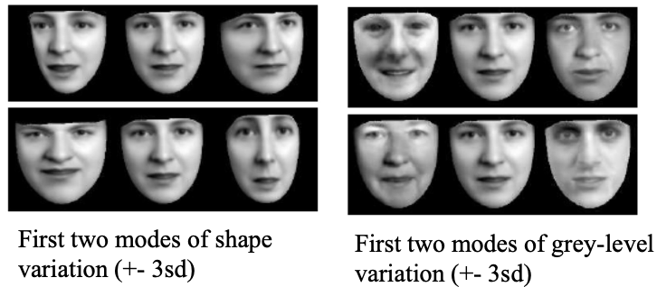
Examples of synthesized faces

Various objects can be synthesized by controlling the parameter $\mathbf{c}$

Dataset for Building Model

IMM data set from Danish Technical University

• 240 images with 640*480 size; 40 individuals, with 36 males and 4 females.

• Each Subject 6 shots, with different pose, expressions and illuminations.

• Each image is labeled with 58 landmarks; 3 closed and 4 opened point-paths.

  

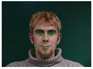
Image Interpretation with Models

• 🎯 Goal: find the set of parameters which best match the model to the image
  • Optimize some cost function
  • Difficult optimization problem
• Set of parameters
  • Defines shape, position, appearance
  • Can be used for further processing

    • Position of landmarks

    • Face recognition

    • Facial expression recognition

    • Pose estimation

• Problem: Optimizing the model fit
  • Active Shape Models
  • Active Appearance Models

Active Shape Models (ASM)

Given a rough starting position, create an instance of $\mathbf{X}$ of the model using

• shape parameters $b$
• translation $T=(X\_t,Y\_t)$
• scale $s$
• rotation $\theta$

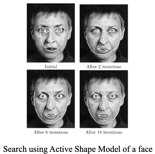
Iterative approach:

1. Examine region of the image around $\mathbf{X}\_i$ to find the best nearby match for the point $\mathbf{X}\_i^\prime$
2. Update parameters $(b, T, s, \theta)$ to best fit the new points $\mathbf{X}$ (constrain the model parameters to be within three standard deviations)
3. Repeat until convergence

In practice: search along profile normals

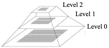
• The optimal parameters are searched from multi-resolution images hierarchically (faster algorithm)

  1. Search for the object in a coarse image
  2. Refine the location in a series of higher resolution images.

  

Example of search

Disadvantages

• Uses mainly shape constraints for search

• Does not take advantage of texture across the target

Active Appearance Models (AAM)

• Optimize parameters, so as to minimize the difference of a synthesized image and the target image
• Solved using a gradient-descent approach

Fitting AAMs

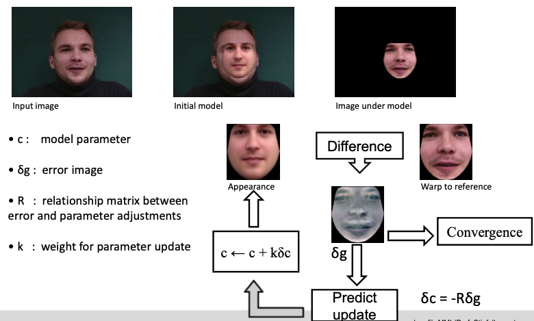
Learning linear relation matrix $\mathbf{R}$ using multi-variate linear regression

• Generate training set by perturbing model parameters for training images

• Include small displacements in position, scale, and orientation

• Record perturbation and image difference

• Experimentally, optimal perturbation around 0.5 standard deviations for each parameter

ASM vs. AAM

ASM

• Seeks to match a set of model points to an image, constrained by a statistical model of shape
• Matches model points using an iterative technique (variant of EM-algorithm)
• A search is made around the current position of each point to find a nearby point which best matches texture for the landmark
• Parameters of the shape model are then updated to move the model points closer to the new points in the image

AAM: matches both position of model points and representation of texture of the object to an image

• Uses the difference between current synthesized image and target image to update parameters
• Typically, less landmark points are needed

Summary of ASM and AAM

• Statistical appearance models provide a compact representation

• Can model variations such as different identities, facial expression, appearances, etc.

• Labeled training images are needed (very time-consuming) 🤪

• Original formulation of ASM and AAM is computationally expensive (i.e. slow) 🤪

• But, efficient extensions and speed-ups exist!

  • Multi-resolution search
  • Constrained AAM search
  • Inverse compositional AAMs (CMU)

• Usage

  • Facial fiducial point detection
  • Face recognition, pose estimation
  • Facial expression analysis
  • Audio-visual speech recognition

More Modern Approaches: Conditional Random Forests For Real Time Facial Feature Detection¹

Basics

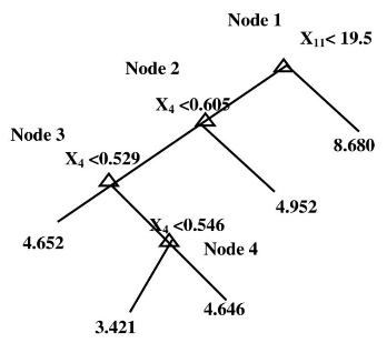
Regression tree

• Basically like classification decision tree

• In the nodes-decisions are comparison of numbers

• In the leafs-numbers or multidimensional vectors of numbers

• Example

  

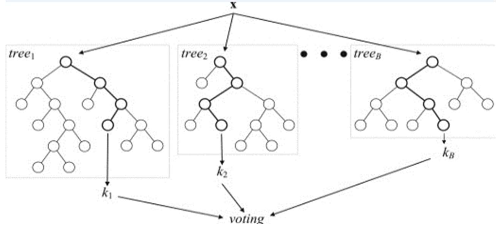
Random regression forests

• Set of random regression trees

• Random

  • Different trees trained on random subset of training data

  • After training, predictions for unseen samples can be made by averaging the predictions from all the individual regression trees

    

Basic idea

• Train different set of trees for different head pose.

• The leaf nodes accumulates votes for the different facial fiducial points

Regression forests training

• Each Tree is trained from randomly selected set of images.

• Extract patches in each image

• Training goal: accumulate probability for a feature point $C\_n$ given a patch $P$ at the leaf node

  • Each patch is represented by appearance features $I$, and displacement vectors $D$ (offsets) to each of the facial fiducial feature point. I.e. $P = \\{I, D\\}$
  • A simple patch comparison is used as Tree-node splitting criterion

Regression forests testing

• Given: a random face image
• Extract densely set of patches from the image
• Feed all patches to all trees in the forest
• Get for each patch $P\_i$ a corresponding set of leafs
• A density estimator for the location of ffp’s is calculated
• Run meanshift to find all locations

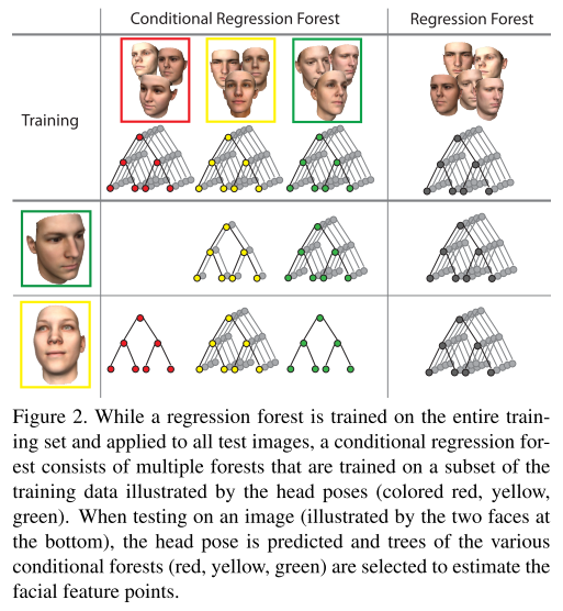
Conditional Regression Forest

• Conditional regression tree works alike.

• For training:

  • Compute a probability for a concrete head pose

  • For each head pose divide the training set in disjoint subsets according to the pose

  • Train a regression forest for each subset

• For testing:

  • Estimate the probabilities for each head pose

  • Select trees from different regression forests

  • Estimate the density function for all facial feature points.

  • Finalize the exact poition by clustering over all feature candidate votes for a given facial feature point. (e.g., by meanshift)

Experiments and results

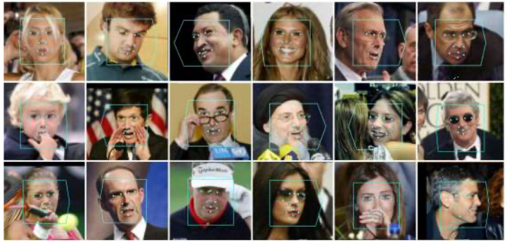
• Training set:

  • 13233 face images from LFW Database
  • 10 annotated facial feature points per face image

• Training

  • Maximum tree depth = 20
  • 2500 splitting candidates and 25 thresholds per split
  • 1500 images to train each tree
  • 200 patches per image (20 * 20 pixels).
  • For head pose two different subsets with 3 and 5 head poses are generated (accuracy 72,5%)
  • Required time for face detection and head pose estimation is 33 ms.

• Results

  

CNN based models

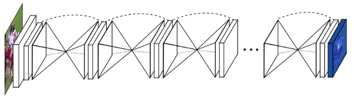
Stacked Hourglass Network ²

• Fully-convolutional neural network

• Repeated down- and upsampling + shortcut connections

• Based on RGB face image, produce one heatmap for each landmark

• Heatmaps are transformed into numerical coordinates using DSNT