People Detection: Global Approaches

Motivation

Why people detection?

• Person Re-Identification

• Person Tracking

• Security (e.g. Border Control)

• Automotive (e.g. Collision Prevention)

• Interaction (e.g. Xbox Kinect)

• Medical (e.g. Patient Monitoring)

• Commercial (e.g. Customer Counting)

Why is people detection difficult?

• Clothing

  Large variety of clothing styles causes greater appearance variety

• Accessories Occlusions by accessories. E.g. backpack, umbrella, handbag, …

• Articulation Faces are mostly rigid. Persons can take on many different poses

• Clutter People frequently overlap each other in images (crowds)

Categories

Still image vs. video

Still image based

• Mostly based on gray-value information from visual images
• Other possible cues: color, infra-red, radar, stereo
• 👍 Advantage: Applicable in wider variety of applications
• 👎 Disadvantages
  • Often more difficult (only a single frame)
  • Performs poorer than video based techniques

Video based

• Background modeling

• Temporal information (speed, position in earlier frames)

• Optical flow

• Can be (re-)initialized by still image approach

• 👎 Disadvantage: Hard to apply in unconstrained scenarios

Global vs. parts

Global approaches

• Holistic model, e.g. one feature for whole person

  

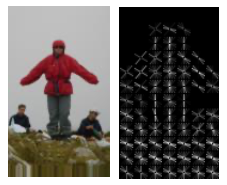
• 👍 Advantages

  • typically simple model
  • work well for low resolutions

• 👎 Disadvantages

  • problems with occlusions
  • problems with articulations

Part-based approaches

• Model body sub-parts separately

  

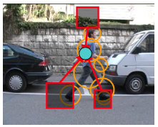
• 👍 Advantages

  • deal better with moving body parts (poses)
  • able to handle occlusions, overlaps
  • sharing of training data

• 👎 Disadvantages

  • require more complex reasoning
  • problems with low resolutions

discriminative vs. generative

Generative model

• Models how data (i.e. person images) is generated

• 👍 Advantages

  • possibly interpretable, i.e. know why reject/accept
  • models the object class/can draw samples

• 👎 Disadvantages

  • model variability unimportant to classification task
  • often hard to build good model with few parameters

Discriminative model

• Can only discriminate for given data, if it is a person or not

• 👍 Advantages

  • appealing when infeasible to model data itself
  • currently often excel in practice

• 👎 Disadvantages

  • often can’t provide uncertainty in predictions
  • non-interpretable

Typical components of global approaches

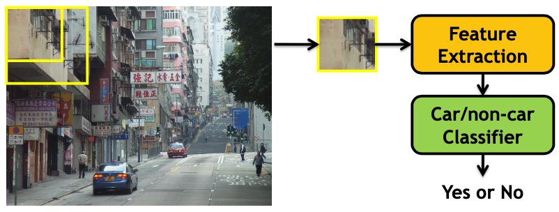
Detection via classification (binary classifier)

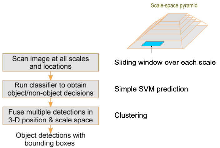
Sliding window: Scan window at different positions and scales

Gradient based

• Popular and successful in the vision community

• Avoid hard decisions (compared to edge based features)

• Examples

  • Histogram of Oriented Gradients (HOG)
  • Scale-Invariant Feature Transform (SIFT)
  • Gradient Location and Orientation Histogram (GLOH)

• Computing gradients

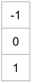
  • Centered

    $$ f^{\prime}(x)=\lim \_{h \rightarrow 0} \frac{f(x+h)-f(x-h)}{2 h} $$

  • Gradient magnitude

    $$ s = \sqrt{s\_x^2 + s\_y^2} $$

  • Gradient orientation

    $$ \theta=\arctan \left(\frac{s\_{y}}{s\_{x}}\right) $$

    

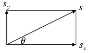
• Gradient in image

  • Image: discrete, 2-dimensional signal

  • Use filter mask to compute gradient

    • $x$-direction:

      

    • $y$-direction

      

Edge based

Wavelet based

HOG people detector ¹

More see: Histogram of Oriented Gradients (HOG)

• Gradient-based feature descriptor developed for people detection
• Global descriptor for the complete body
• High-dimensional (typically ~4000 dimensions)
• Very promising results on challenging data sets

Phases

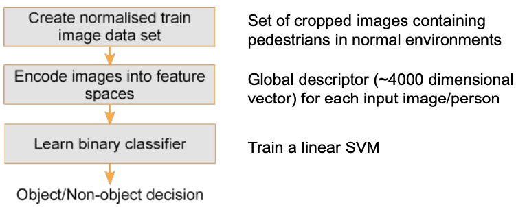
Learning Phase

Detection Phase

How HOG descriptor works?

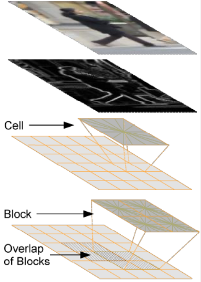
1. Compute gradients on an image region of 64x128 pixels
2. Compute gradient orientation histograms on cells of 8x8 pixels (in total 8x16 cells). typical histogram size: 9 bins
3. Normalize histograms within overlapping blocks of 2x2 cells (in total 7x15 blocks) block descriptor size: 4x9 = 36
4. Concatenate block descriptors $\rightarrow$ 7 x 15 x 4 x 9 = 3780 dimensional feature vector

1. Gradients

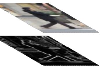
• Convolution with [-1 0 1] filters (x and y direction)

• Compute gradient magnitude and direction

  • Per pixel: color channel with greatest magnitude is used for final gradient (color is used!)

    

2. Cell histograms

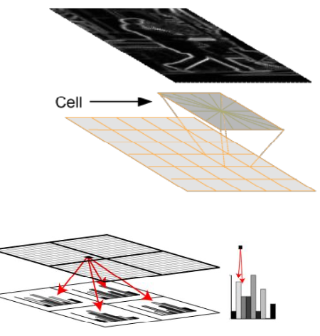
• 9 bins for gradient orientations (0-180 degrees)
• Filled with magnitudes
• Interpolated trilinearly
  • bilinearly into spatial cells
  • linearly into orientation bins

3. Blocks

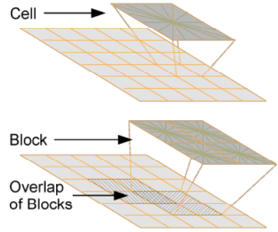
• Overlapping blocks of 2x2 cells
• Cell histograms are concatenated and then normalized
• Normalization
  • different norms possible (L2, L2hys etc.)
  • add a normalization epsilon to avoid division by zero

4. The final HOG descriptor

Concatenation of block descriptors

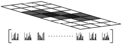
Visualization

From feature to detector

• Simple linear SVM on top of the HOG Features

  • Fast (one inner product per evaluation window)

    for an entire image it’s a vector-matrix multiplication

• Gaussian kernel SVM

  • slightly better classification accuracy

  • but considerable increase in computation time

Silhouette Matching ²

Idea

• 🎯 Goal: align known object shapes with image

  

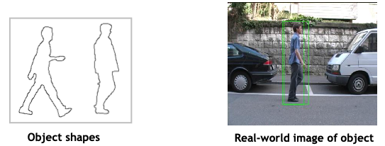
• Requirements for an alignment algorithm

  • high detection rate

  • few false positives

  • robustness

  • computationally inexpensive

Computational complexity

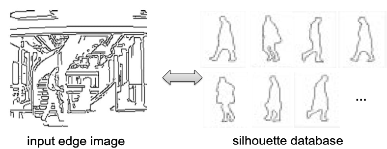
Complexity is O(#positions * #templates * #contourpixels * sizeof(searchregion))

Distance transform

Used to compare/align two (typically binary) shapes

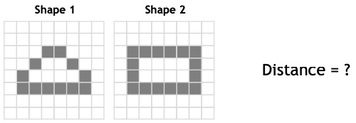
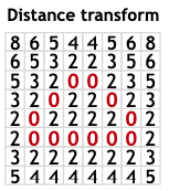
1. Compute the distance from each pixel to the nearest edge pixel

   • here the euclidean distances are approximated by the 2-3 distance
   

2. Overlay second shape over distance transform

   

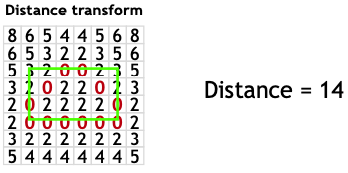
3. Accumulate distances along shape 2

4. Find best matching position by an exhaustive search

However:

• 2-3 distance is not symmetric
• 2-3 distance has to be normalized w.r.t. the length of the shapes

Chamfer matching

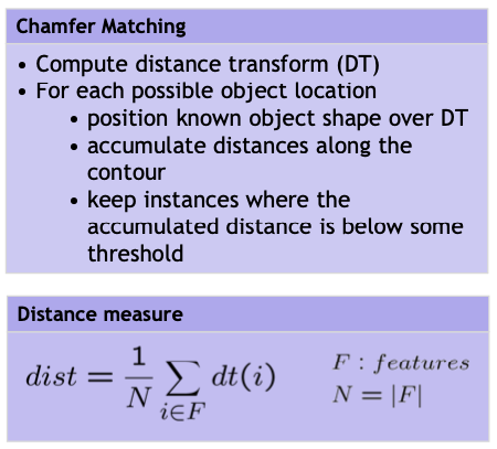
Efficient Implementation

The distance transform can be efficiently computed by two scans over the complete image

• Forward-Scan

  • starts in the upper-left corner and moves from left to right, top to bottom

  • uses the following mask

    

• Backward-Scan

  • starts in the lower-right corner and moves from right to left, bottom to top

  • uses the following mask

    

Advantages

• Fast
• Good performance on uncluttered images (with few background structures)

Disadvantages

• Bad performance for cluttered images
• Needs a huge number of people silhouettes

Template Hierarchy

• Reduce the number of silhouettes to consider
• The shapes are clustered by similarity

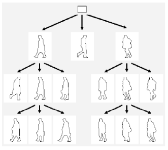
Coarse-To-Fine Search

• Goal: Reduce search effort by discarding unlikely regions with minimal computational effort

• Idea:

  • subsample the image and search first at a coarse scale

  • only consider regions with a low distance when searching for a match on finer scales

• Need to find reasonable thresholds