Body Pose
Kinect
What is Kinect?
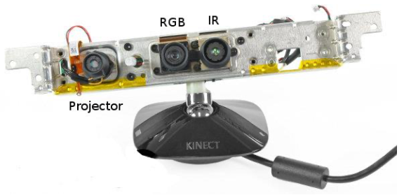
- Fusion of two groundbreaking new technologies
- A cheap and fast RGB-D sensor
- A reliable Skeleton Tracking
Structured light
- Kinect uses Structured Light to simulate a stereo camera system
- Kinect provides an unique texture for every point of the image, therefore only Block-Matching is required
Pose Recognition for User Interaction
Few constrains:
- Extremely low latency.
- Low computational power.
- High recognition rate, without false positives.
- Any personalized training step.
- Few people at once.
- Complex poses will be usual.
Pose Recognition1
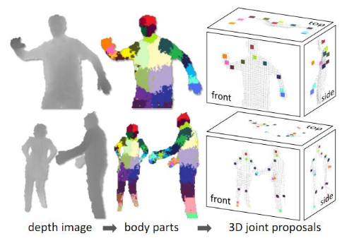
1st step: Pixel classification
Speed is the key
Uses only one disparity image.
It classifies each pixel independently.
The process of feature extraction is simultaneous to the classification.
Simplest possible feature: difference between two pixels.
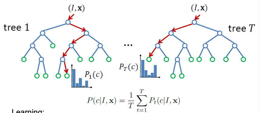
Classification is done through Random Decision Forests.
- Learning
- Randomly choose a set of thresholds and features for splits.
- Pick the threshold and feature that provide the largest information gain.
- Recurse until a certain accuracy is reached or depth is obtained.
- Learning
Everything has an optimal GPU implementation.
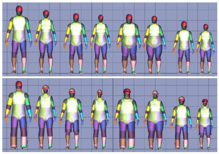
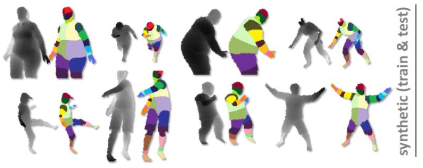
Training
Key: using a huge amount of training data
Synthetic Training DB
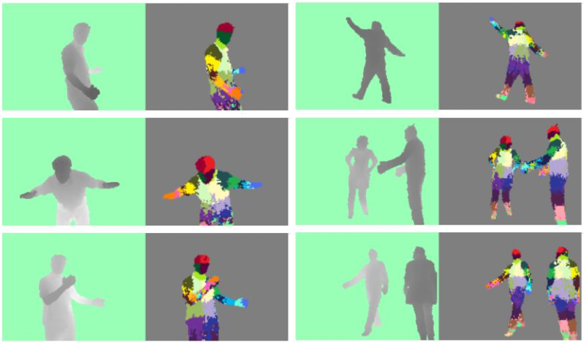
Pixel classification results
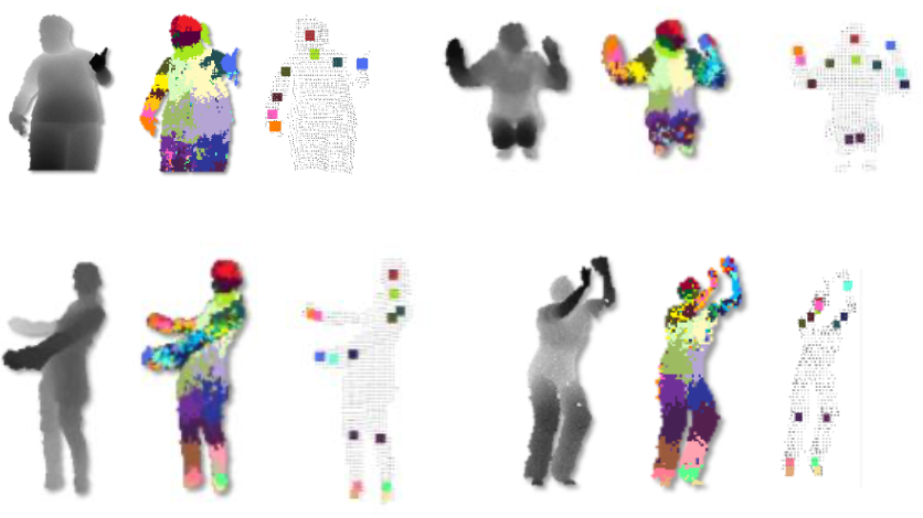
Joint estimation
Use mean shift clustering on the pixels with Gaussian kernel to infer the center of clusters.
Clustering is done in 3d space but every pixel is weighted by their world surface area to get depth invariance.
Finally the sum of the weighted pixels is used as a confidence measure.
Results
Criticism 👎
- Not open source
- Biased towards upper body frontal poses
- Very difficult to improve or adapt.
Pose Estimation without Kinect: Convolutional Pose Machines 2
Pose Machine
Unconstrained 2D-pose estimation on real world RGB images.
Outputs confidence maps for every joint of the skeleton.
Works in multiple stages refining the confidence maps.
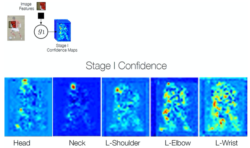
💡 Idea:
Local image evidence is weak (first stage confidence maps)
Part context can be a strong cue (confidence maps of other body joints)
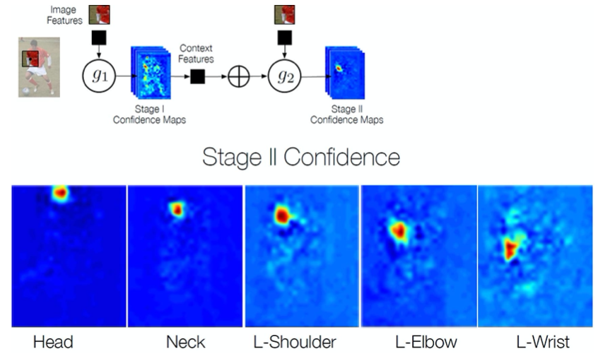
➔ Use confidence maps of all body joints of the previous stage to refine current results
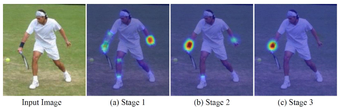
Example
Details
We denote the pixel location of the $p$-th anatomical landmark (refer to as a part) $Y\_{p} \in \mathcal{Z} \subset \mathbb{R}^{2}$
- $\mathcal{Z}$: set of all $(u, v)$ locations in an image
🎯 Goal: to predict the image locations $Y = (Y\_1, \dots, Y\_P)$ for all $P$ parts.
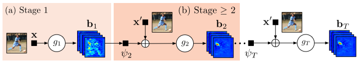
In each stage $t \in \{1 \dots T\}$, the classifiers $g\_t$ predict beliefs for assigning a location to each part $Y\_{p}=z, \forall z \in \mathcal{Z}$, based on
- features extracted from the image at the location $z$ denoted by $\mathbf{x}\_{z} \in \mathbb{R}^{d}$ and
- contextual information from the preceding classifier in the neighborhood around each $Y\_p$ in stage $t$.
First stage
A classifier in the first stage $t = 1$ produces the following belief values:
$$ g\_1(\mathbf{x}\_z) \rightarrow \\{b\_1^p(Y\_p=z)\\}\_{p \in \\{0 \dots P\\}} $$- $b\_{1}^{p}\left(Y\_{p}=z\right)$: score predicted by the classifier $g\_1$ for assigning the $p$-th part in the first stage at image location $z$.
We represent all the beliefs of part $p$ evaluated at every location $z = (u, v)^T$ in the image as $\mathbf{b}\_{t}^{p} \in \mathbb{R}^{w \times h}$:
$$ \mathbf{b}\_{t}^{p}[u, v]=b\_{t}^{p}\left(Y\_{p}=z\right) $$- $w, h$: width and height of the image, respectively
For convenience, we denote the collection of belief maps for all the parts as $\mathbf{b}\_{t} \in \mathbb{R}^{w \times h \times(P+1)}$ ($+1$ for background)
Subsequent stages
The classifier predicts a belief for assigning a location to each part $Y\_{p}=z, \forall z \in \mathcal{Z}$, based on
- features of the image data $\mathbf{x}\_{z}^{t} \in \mathbb{R}^{d}$ and
- contextual information from the preceeding classifier in the neighborhood around each $Y\_p$
- $\psi\_{t>1}(\cdot)$: mapping from the beliefs $b\_{t−1}$ to context features.
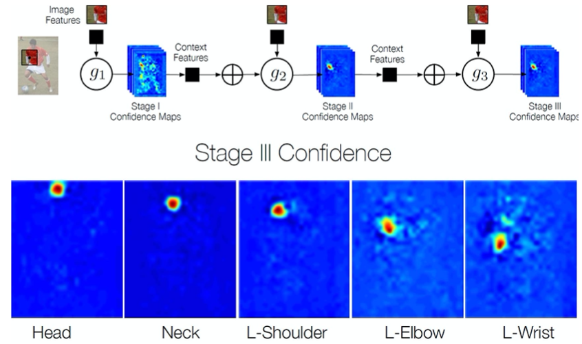
In each stage, the computed beliefs provide an increasingly refined estimate for the location of each part.
Confidence maps generation
Fully Convolutional Network (FCN)
- Does not have Fully Connected Layers.
- The same network can be applied to arbitrary image sizes.
- Similar to a sliding window approach, but more efficient
CPM
The prediction and image feature computation modules of a pose machine can be replaced by a deep convolutional architecture allowing for both image and contextual feature representations to be learned directly from data.
Advantage of convolutional architectures: completely differentiale $\rightarrow$ enabling end-to-end joint trainining of all stages 👍
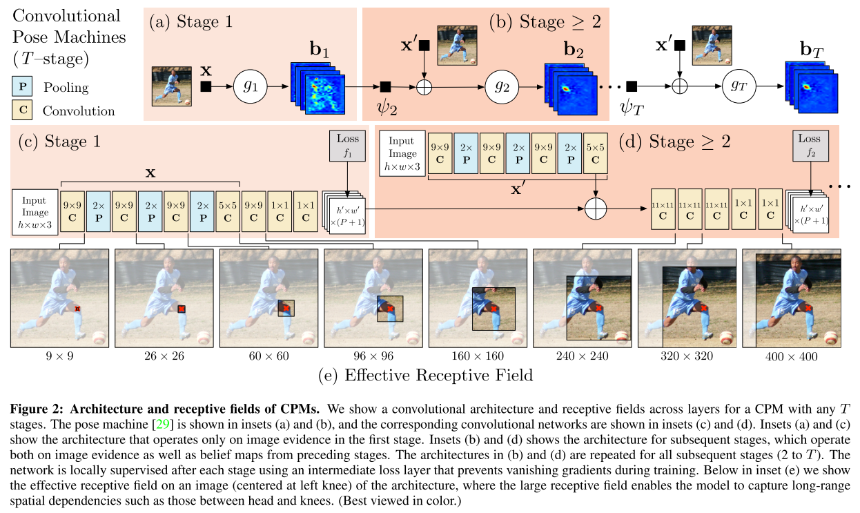
CPM structure
Learning in CPM
Potential problem of a network with a large number of layers: vanishing gradient
Solution
Define a loss function at the output of each stage $t$ that minimizes the $l_2$ distance between the predicted ($b\_{t}^{p}$) and ideal ($b\_{*}^{p}\left(Y\_{p}=z\right)$) belief maps for each part.
- The ideal belief map for a part $p$, $b\_{*}^{p}\left(Y\_{p}=z\right)$, are created by putting Gaussian peaks at ground truth locations of each body part $p$.
Cost function we aim to minimize at the output of each stage at each level:
$$ f\_{t}=\sum\_{p=1}^{P+1} \sum\_{z \in \mathcal{Z}}\left\|b\_{t}^{p}(z)-b\_{*}^{p}(z)\right\|\_{2}^{2} . $$- $P$: all body parts
- $\mathcal{Z}$: set of all image locations in a believe map
The overall objective for the full architecture is obtained by adding the losses at each stage:
$$ \mathcal{F}=\sum\_{t=1}^{T} f\_{t} $$
J. Shotton et al., “Real-time human pose recognition in parts from single depth images,” CVPR 2011, 2011, pp. 1297-1304, doi: 10.1109/CVPR.2011.5995316. ↩︎
Shih-En Wei, Varun Ramakrishna, Takeo Kanade, and Yaser Sheikh. Convolutional pose machines. In Proceedings of the IEEE Conference on Computer Vision and Pattern Recognition (CVPR), pages 4724–4732, 2016 ↩︎