Imagine those as three 2d-matrices stacked over each other (one for each color), each having pixel values in the range 0 to 255.
We can consider channel as depth of the image.
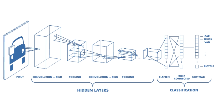
Convolutional Layer
Convolution operation
Extract features from the input image and produce feature maps
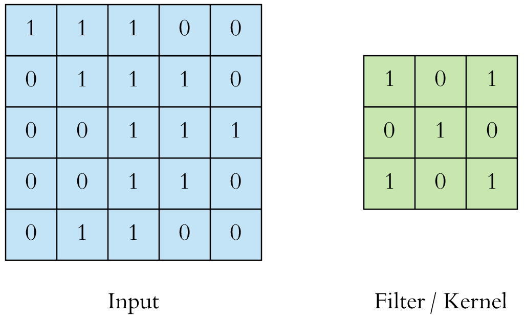
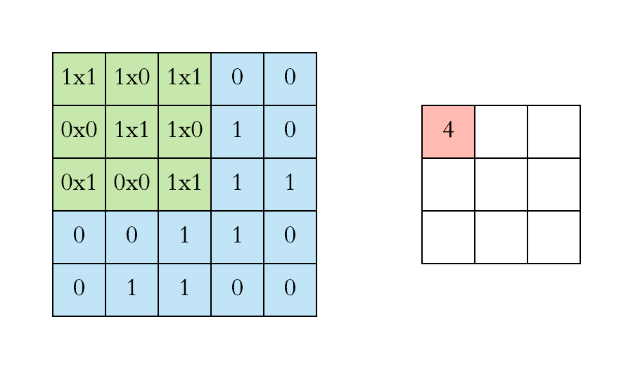
Slide the convonlutional filter/kernel over the input image
At every location, do element-wise matrix multiplication and sum the result.
This can preserve the spatial relationship between pixels by learning image features using small squares of input data 👍
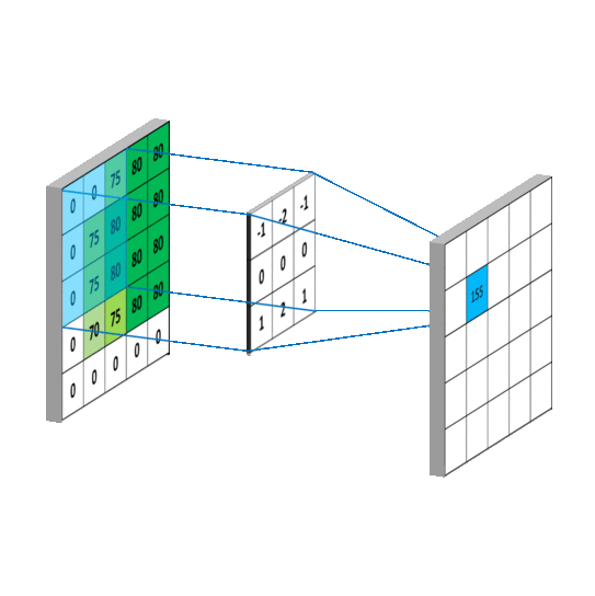
2D Convolution
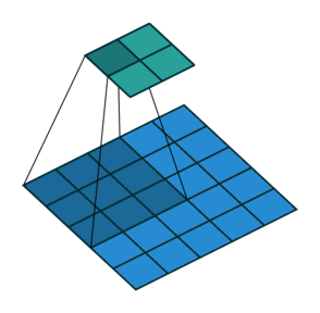
Convolution operation in 2D using a $3\times3$ filter
Another example:
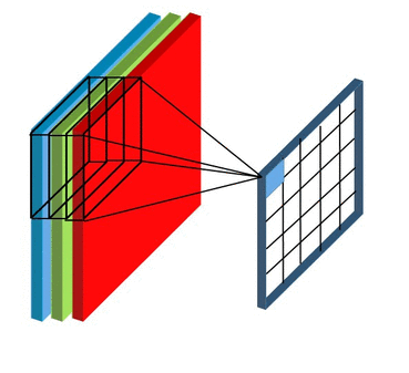
3D Convolution
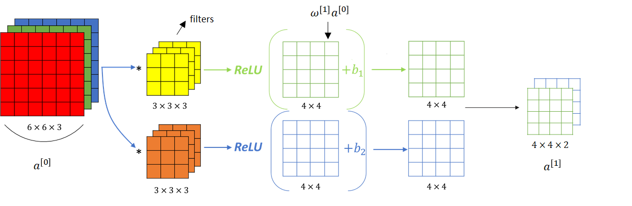
In reality an image is represented as a 3D matrix with dimensions of height, width and depth, where depth corresponds to color channels (RGB). A convolution filter has a specific height and width, like $3 \times 3$ or $5 \times 5$, and by design it covers the entire depth of its input ($\text{depth}\_{\text{filter}} = \text{depth}\_{\text{input}}$).
The convolution filter/kernel has the same depth as the input image
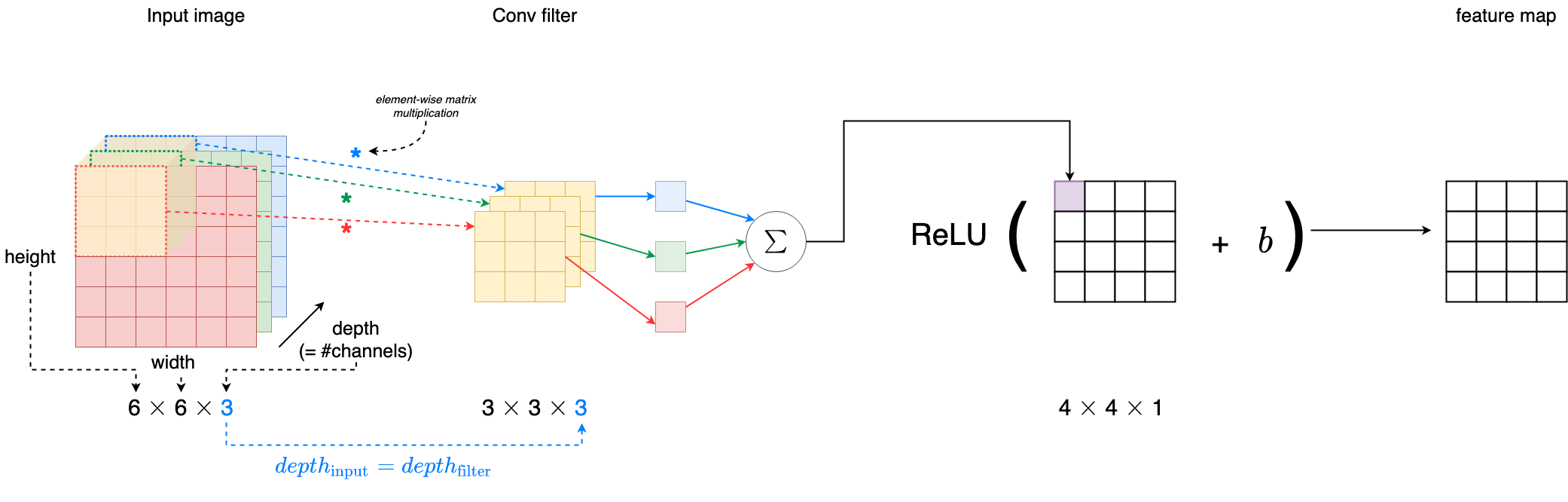
Convolution using a single filter:
Convolution using a single filter
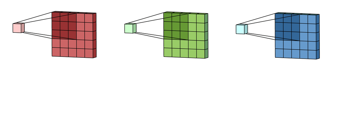
Each filter actually happens to be a collection of kernels, with there being one kernel for every single input channel to the layer, and each kernel being unique. As the input image has 3 channels (RGB), our filter consists of also 3 kernels.
Each of the kernels of the filter “slides” over their respective input channels, producing a processed version of each.
Each of the per-channel processed versions are then summed together to form one channel. The kernels of a filter each produce one version of each channel, and the filter as a whole produces one overall output channel.
We can stack different filters to obtain a multi-channel output “image”.
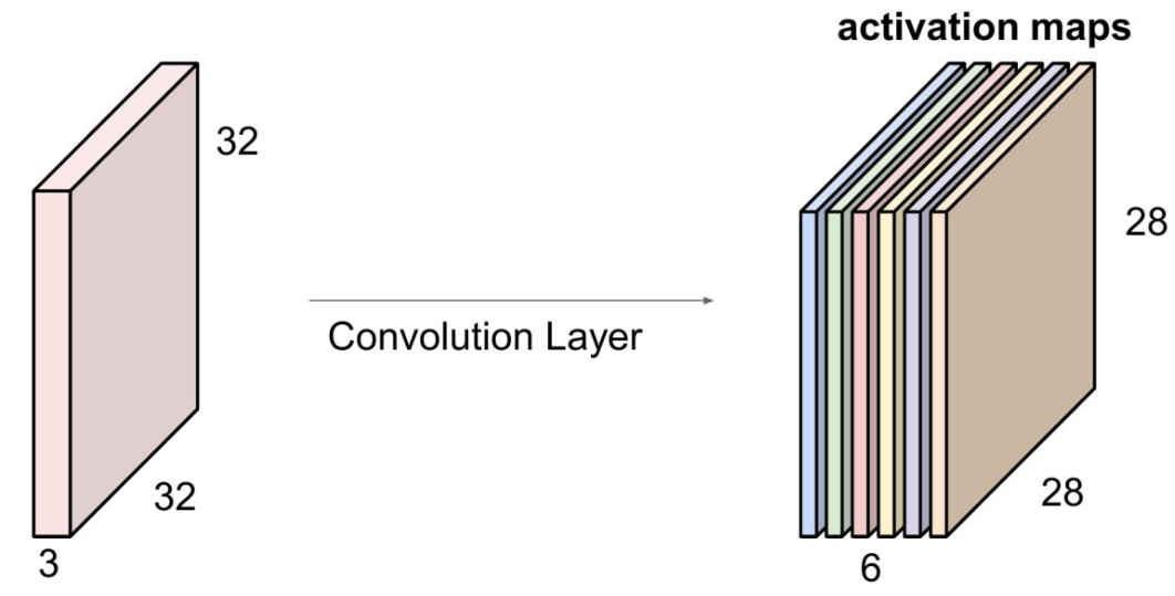
For example, assuming that
input image has the size $\text{height} \times \text{width} \times \text{depth} = 32 \times 32 \times 3$
filter size is $5 \times 5 \times 3$
and we have 6 different filters
$\to$ we’ll get 6 separate activation maps and stack it together
$\Rightarrow$ The depth of the multi-channel output “image” is 6.
($depth\_\text{activation maps} = \\# filters$)
Convolution Example
A filter (with red outline) slides over the input image (convolution operation) to produce a feature map. The convolution of another filter (with the green outline), over the same image gives a different feature map as shown. It is important to note that the Convolution operation captures the local dependencies in the original image. Also notice how these two different filters generate different feature maps from the same original image.
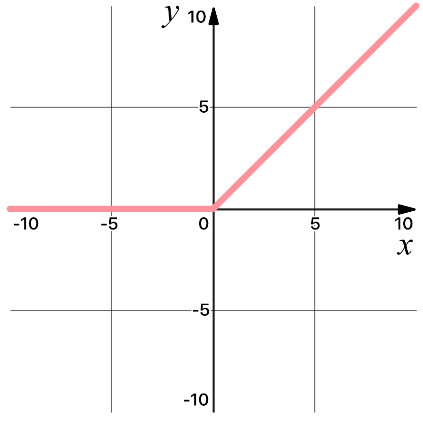
Non-linearity: ReLU
For any kind of neural network to be powerful, it needs to contain non-linearity. And CNN is no different.
After the convolution operation, we pass the result through non-linear activation function. In CNN we usually use Rectified Linear Units (ReLU), because it has been empirically observed that CNNs using ReLU are faster to train than their counterparts.
$$
\operatorname{ReLU}(x) = \max(0, x)
$$
ReLU Example
This example shows the ReLU operation applied to one of the fearure maps obtained in the convolutional example. The output feature map here is also referred to as the ‘Rectified’ feature map.
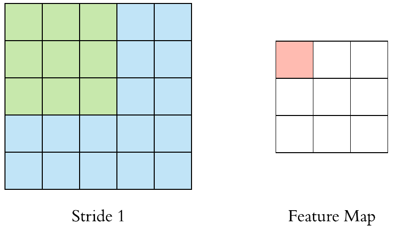
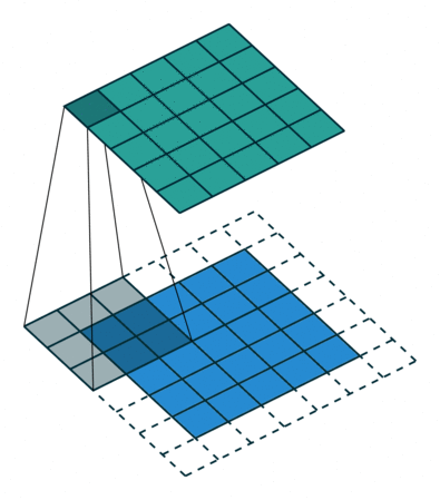
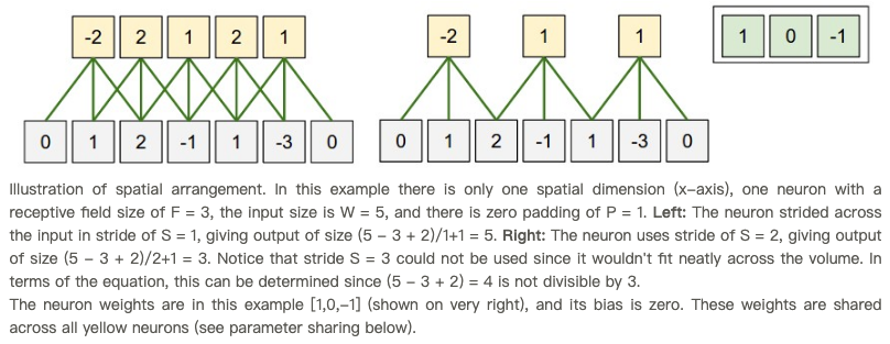
Stride and Padding
Stride specifies how much we move the convolution filter at each step.
By default the value is 1:
Stride > 1often used to down-sample the image
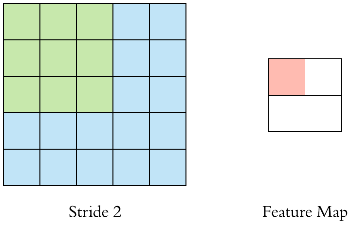
Stride 2 convolution
What do we do with border pixels?
$\to$ Paddings
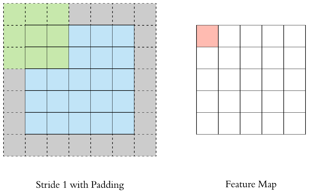
Fill up the image borders (zero-padding is most common)
Preserve the size of the feature maps from shrinking
Improves performance and makes sure the kernel and stride size will fit in the input
Height and width of feature map is same as the input image due to padding (the gray area).
After a convolution operation we usually perform pooling to reduce the dimensionality.
Pooling layers downsample each feature map independently, reducing the height and width, keeping the depth intact. This enables us to reduce the number of parameters, which both shortens the training time and combats overfitting. 👏
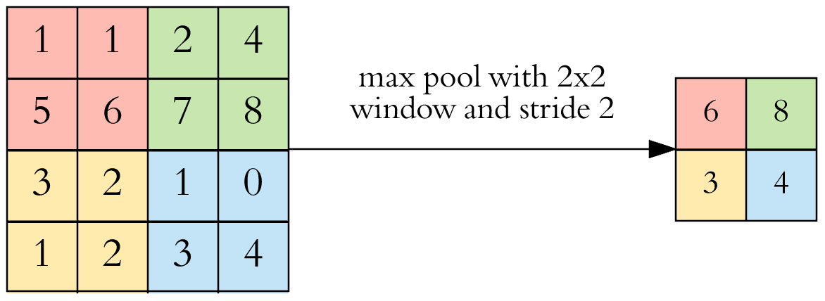
The most common type of pooling is max pooling which just takes the max value in the pooling window. Contrary to the convolution operation, pooling has NO parameters. It slides a window over its input, and simply takes the max value in the window. Similar to a convolution, we specify the window size and stride.
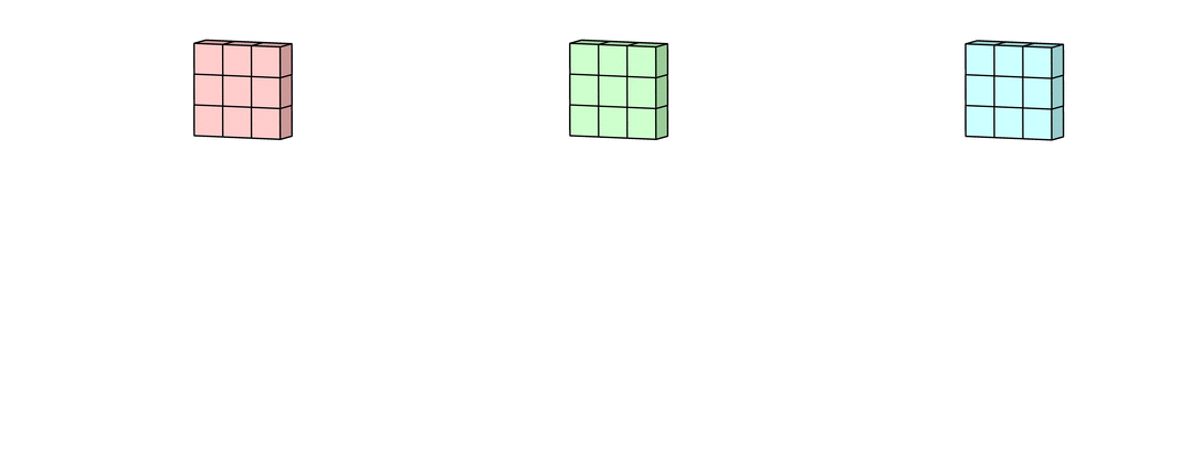
Example: max pooling using a $2 \times 2$ window and stride 2
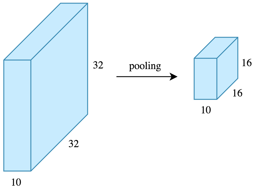
Now let’s work out the feature map dimensions before and after pooling.
If the input to the pooling layer has the dimensionality $32 \times 32 \times 10$, using the same pooling parameters described above, the result will be a $16 \times 16 \times 10$ feature map.
Both the height and width of the feature map are halved. Thus we reduced the number of weights to 1/4 of the input.
The depth doesn’t change because pooling works independently on each depth slice the input.
In CNN architectures, pooling is typically performed with 2x2 windows, stride 2 and NO padding.
Pooling Example
This example shows the effect of Pooling on the Rectified Feature Map we received after the ReLU operation in the above ReLU example. Max refers to Max-Pooling and Sum refers to Sum-Pooling.
Why pooling works?
Because Pooling keeps the maximum value from each window, it preserves the best fits of each feature within the window. This means that it doesn’t care so much exactly where the feature fit as long as it fit somewhere within the window.
The result of this is that CNNs can find whether a feature is in an image without worrying about where it is. This helps solve the problem of computers being hyper-literal.
In particular, Pooling
makes the input representations (feature dimension) smaller and more manageable
reduces the number of parameters and computations in the network, therefore, controlling overfitting
makes the network invariant to small transformations, distortions and translations in the input image (a small distortion in input will not change the output of Pooling – since we take the maximum / average value in a local neighborhood).
helps us arrive at an almost scale invariant representation of our image
Dimension parameters computation
Inpupt size:
$$W\_{1} \times H\_{1} \times D\_{1}$$
(usually $W\_1 = H\_1$)
Hyperparameters:
Number of filters: $K$
Filter size: $F \times F \times D\_1$
Stride: $S$
Typically no padding
Output size:
$$
W\_{2} \times H\_{2} \times D\_1
$$
with
$W_{2}=\lfloor \frac{W_{1}-F}{S}\rfloor+1 $
$H_{2}=\lfloor \frac{H_{1}-F}{S}\rfloor+1 $
Number of weights: 0 (since it computes a fixed function of the input)
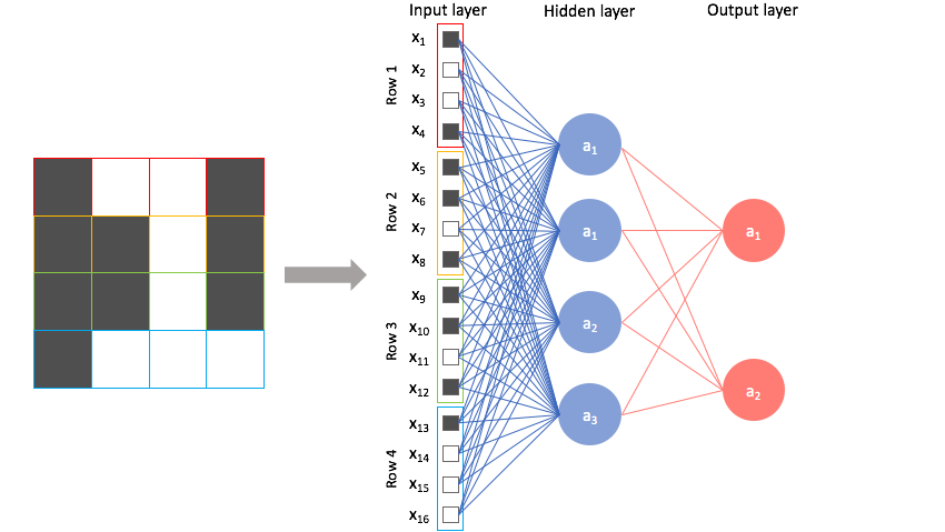
Fully Connected Layer
After the convolution + pooling layers we add a couple of fully connected layers to wrap up the CNN architecture.
The Fully Connected layer is a traditional MultiLayer Perceptron (MLP) that uses a softmax activation function in the output layer (other classifiers like SVM can also be used). The term “Fully Connected” implies that every neuron in the previous layer is connected to every neuron on the next layer.
The output from the convolutional and pooling layers represent high-level features of the input image. The purpose of the Fully Connected layer is to use these features for classifying the input image into various classes based on the training dataset.
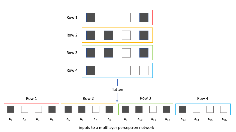
Remember that the output of both convolution and pooling layers are 3D volumes, but a fully connected layer expects a 1D vector of numbers. So we flatten the output of the final pooling layer to a vector and that becomes the input to the fully connected layer. Flattening is simply arranging the 3D volume of numbers into a 1D vector, nothing fancy happens here.