👍 Attention

Core Idea

The main assumption in sequence modelling networks such as RNNs, LSTMs and GRUs is that the current state holds information for the whole of input seen so far. Hence the final state of a RNN after reading the whole input sequence should contain complete information about that sequence. But this seems to be too strong a condition and too much to ask.

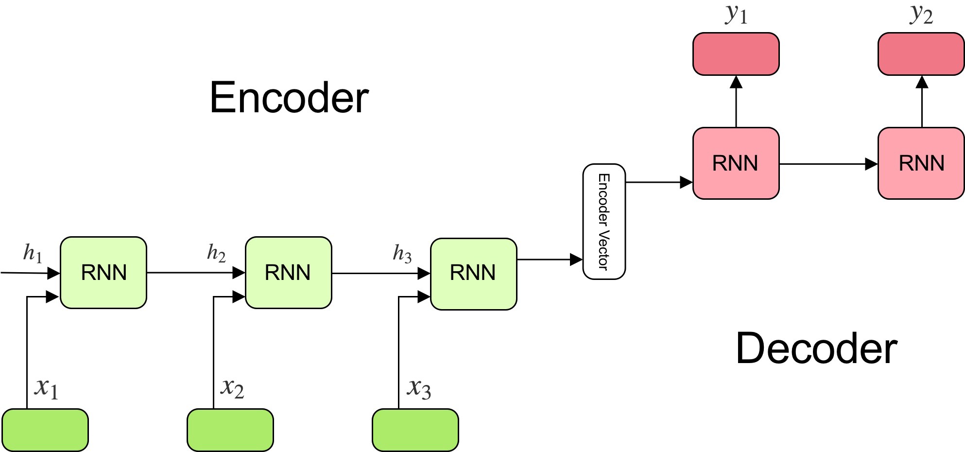
Attention mechanism relax this assumption and proposes that we should look at the hidden states corresponding to the whole input sequence in order to make any prediction.

Details

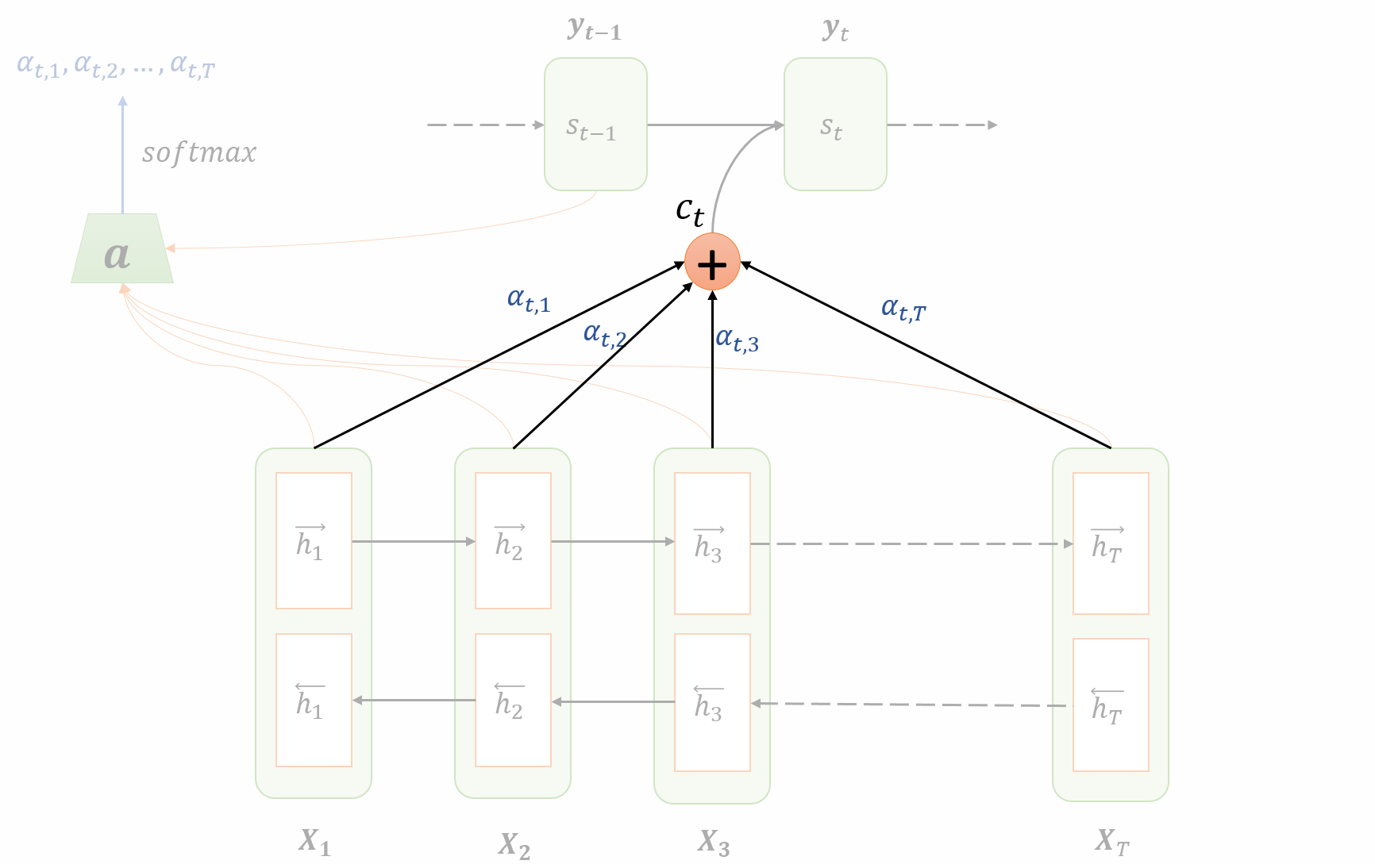
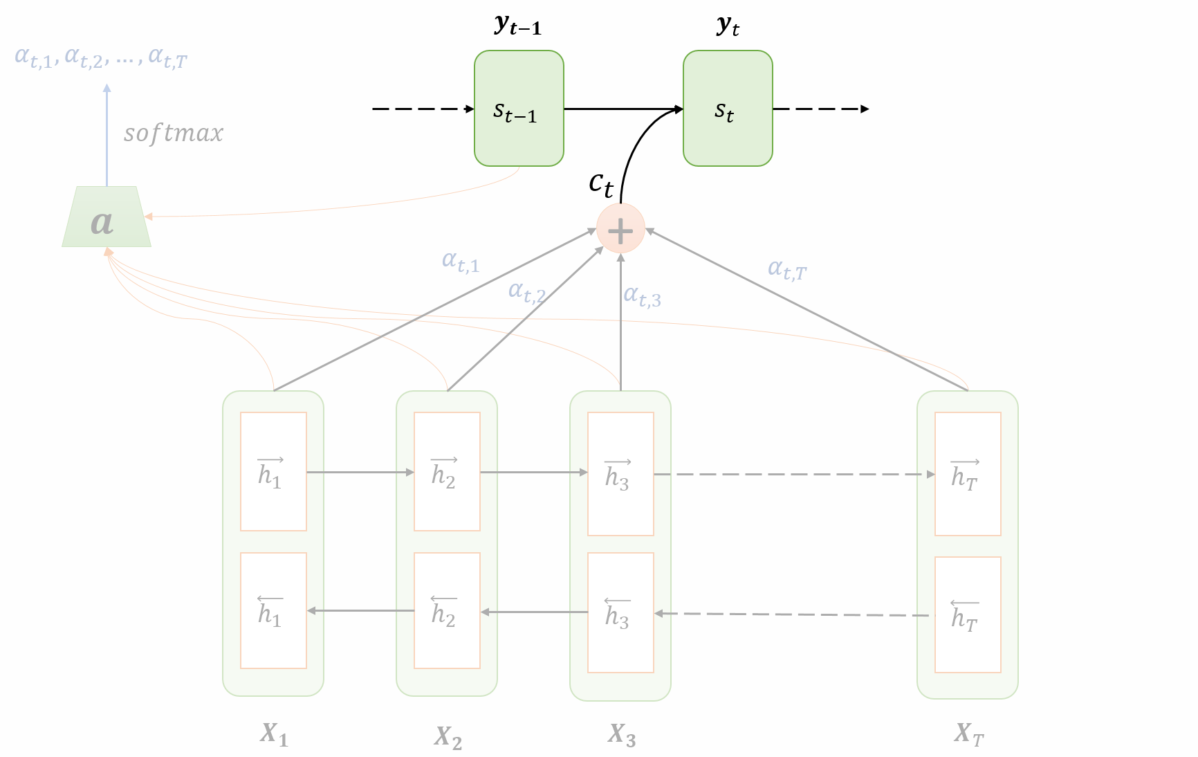
The architecture of attention mechanism:

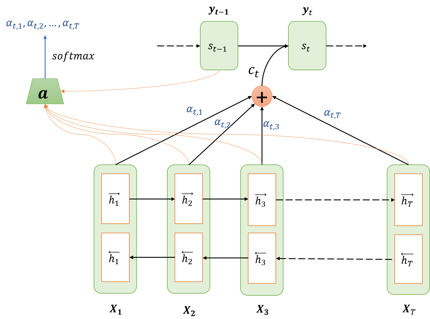
The network is shown in a state:

• the encoder (lower part of the figure) has computed the hidden states $h\_j$ corresponding to each input $X\_j$
• the decoder (top part of the figure) has run for $t-1$ steps and is now going to produce output for time step $t$.

The whole process can be divided into four steps:

1. Encoding
2. Computing Attention Weights/Alignment
3. Creating context vector
4. Decoding/Translation

Encoding

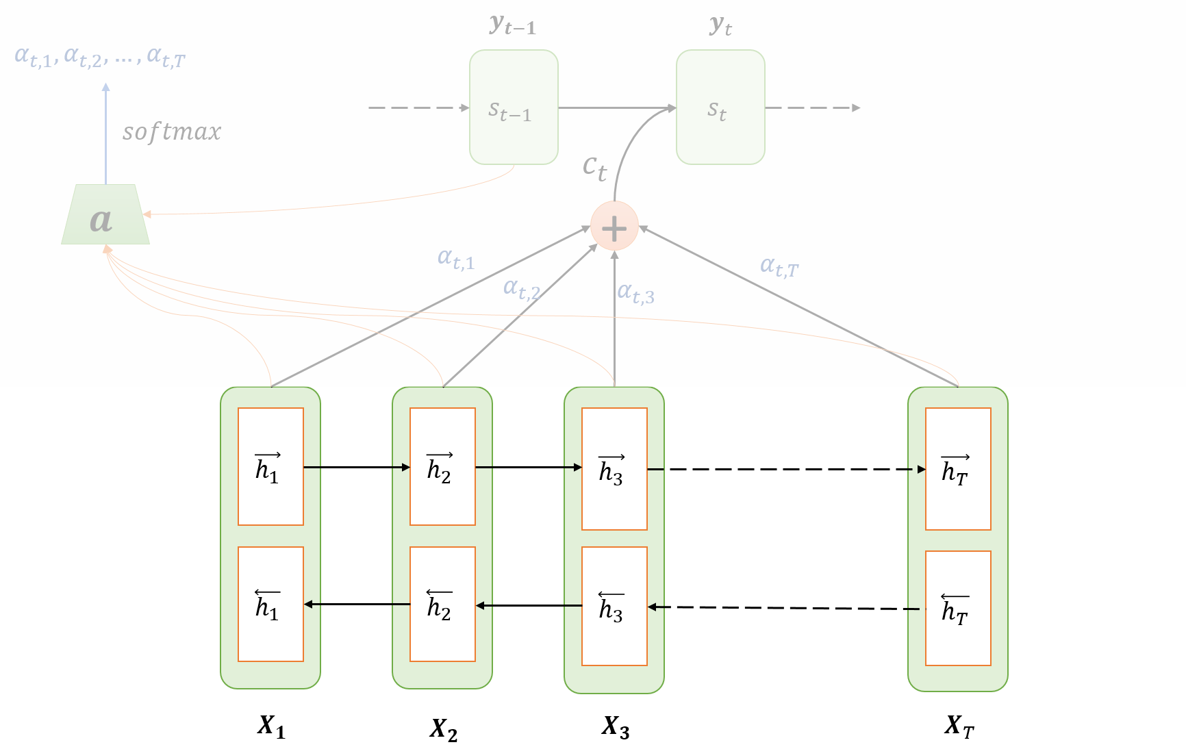
• $(X\_1, X\_2, \dots, X\_T)$: Input sequence

  • $T$: Length of sequence

• $(\overrightarrow{h}\_{1}, \overrightarrow{h}\_{2}, \dots, \overrightarrow{h}\_{T})$: Hidden state of the forward RNN

• $(\overleftarrow{h}\_{1}, \overleftarrow{h}\_{2}, \ldots \overleftarrow{h}\_{T})$: Hidden state of the backward RNN

• The hidden state for the $j$-th input $h\_j$ is the concatenation of $j$-th hidden states of forward and backward RNNs.

  $$h\_{j}=\left[\overrightarrow{h}\_{j} ; \overleftarrow{h}\_{j}\right], \quad \forall j \in[1, T]$$

Computing Attention Weights/Alignment

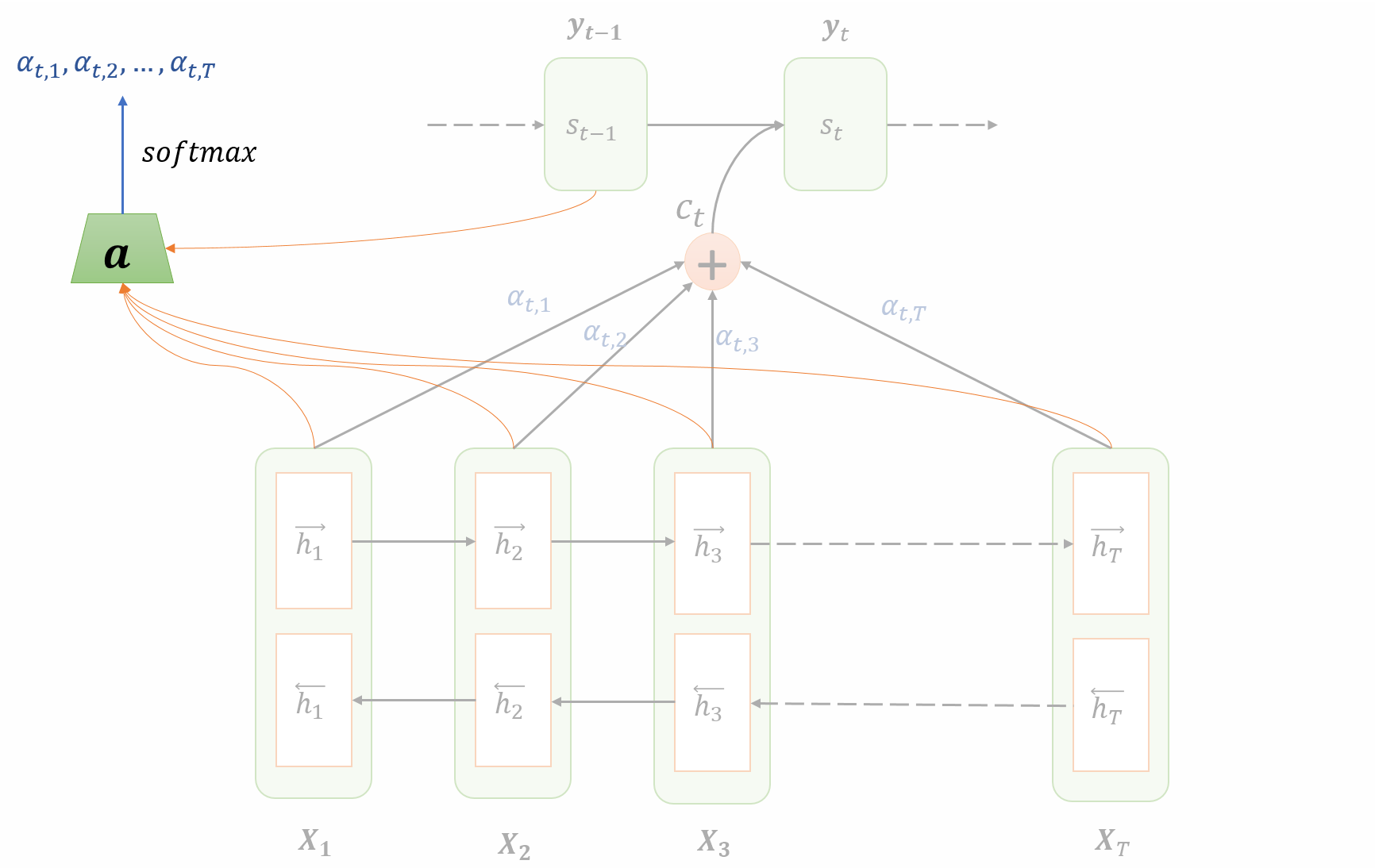
At each time step $t$ of the decoder, the amount of attention to be paid to the hidden encoder unit $h\_j$ is denoted by $\alpha_{tj}$ and calculated as a function of both $h\_j$ and previous hidden state of decoder $s\_{t-1}$:

• $\boldsymbol{a}(\cdot)$: parametrized as a feedforward neural network that runs for all $j$ at the decoding time step $t$
• $\alpha\_{tj} \in [0, 1]$
• $\displaystyle \sum\_j \alpha\_{tj} = 1$
• $\alpha\_{tj}$ can be visualized as the attention paid by decoder at time step $t$ to the hidden ecncoder unit $h\_j$

Computing Context Vector

Now we compute the context vector. The context vector is simply a linear combination of the hidden weights $h\_j$ weighted by the attention values $\alpha_{tj}$ that we’ve computed in the precdeing step:

From the equation we can see that $\alpha_{tj}$ determines how much $h\_j$ affects the context $c\_t$. The higher the value, the higher the impact of $h\_j$ on the context for time $t$.

Decoding/Translation

Compute the new hidden state $s\_t$ using

• the context vector $c\_t$
• the previous hidden state of the decoder $s\_{t-1}$
• the previous output $y\_{t-1}$

The output at time step $t$ is

Reference

• Understanding Attention Mechanism
• Attention and Memory in Deep Learning and NLP
• Visualizing A Neural Machine Translation Model (Mechanics of Seq2seq Models With Attention) 👍