Sequence to Sequence

Language Modeling

Language model is a particular model calculating the probability of a sequence

$$ \begin{aligned} P(W) &= P(W\_1 W\_2 \dots W\_n) \\\\ &= P\left(W\_{1}\right) P\left(W_{2} \mid W\_{1}\right) P\left(W\_{3} \mid W\_{1} W\_{2}\right) \ldots P\left(W\_{n} \mid W\_{1 \ldots n-1}\right) \end{aligned} $$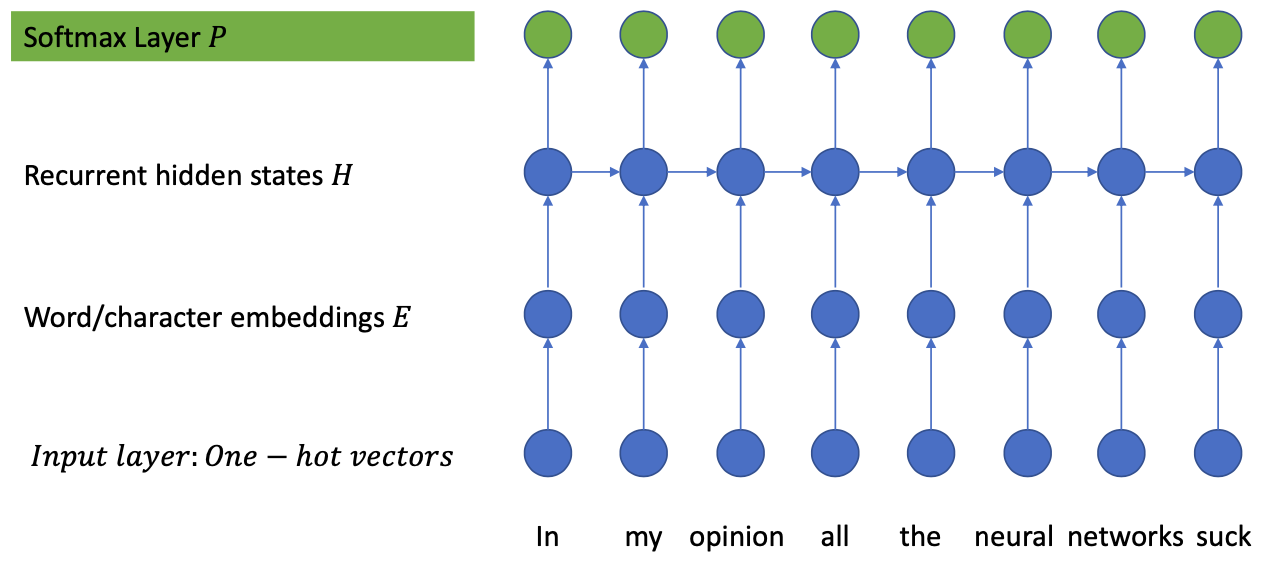

• Softmax layer

  • After linear mapping the hidden layer $H$, a “score” vector $O = [O\_1, O\_2, \dots, O\_{n-1}, O\_n]$ is obtained

  • The softmax function normalizes $O$ to get probabilities

    $$ P\_{i}=\frac{\exp \left(O\_{i}\right)}{\sum\_{j} \exp \left(O\_{j}\right)} $$

• Cross-Entropy Loss

  • Use one-hot-vector $Y = [0,0,0,0,0,\dots,1,0,0]$ as the label to train the model

  • Cross-entropy loss: difference between predicted probability and label

    $$ L\_{CE} = \sum\_i Y\_i \log(P\_i) $$

  • When 𝑌 is an one-hot vector:

    $$ L\_{C E}=-\log P_{j}(\text{the index of the correct word}) $$

Training

Force the model to “fit” known text sequences (teacher forcing / memorization)

• $W=w\_{1} w\_{2} w\_{3} \dots w\_{n-2} w\_{n-1} w\_{N}$
• Input: $w\_{1} w\_{2} w\_{3} \dots w\_{n-2} w\_{n-1}$
• Output: $w\_{2} w\_{3} \dots w\_{n-2} w\_{n-1} w\_{N}$

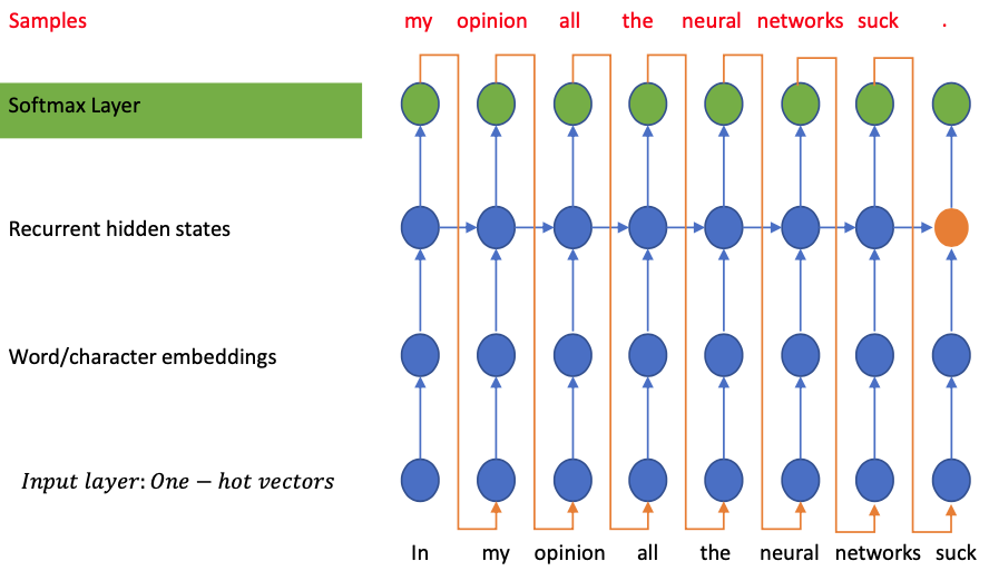
In generation: this model uses its own output at time step $t-1$ as input for time step $t$ (Auto regressive, or sampling mode)

RNN Language Modeling

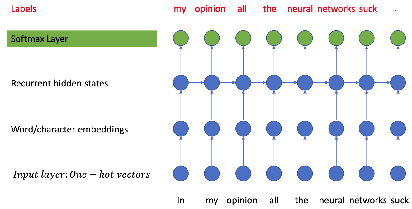
Basic step-wise operation

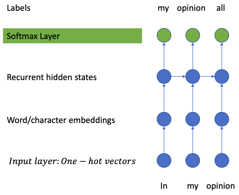
• Input: $x\_t = [0, 0, 0, 1, \dots ]$

• Label: $y\_t = [0, 0, 1, 0, \dots]$

• Input to word embeddings:

  $$ e\_t = x\_t \cdot W\_{emb}^T $$

• Hidden layer:

  $$ h\_t = \operatorname{LSTM}(x\_t, (t\_{t-1}, c\_{t-1})) $$

• Output:

  $$ o\_t = h\_t \cdot W\_{out}^T $$

• Softmax:

  $$ p\_t = \operatorname{softmax}(o\_t) $$

• Loss: Cross Entropy

  $$ L\_t = \sum\_i y\_{t\_{i}} \log p(y\_{t\_{i}}) $$

  ($y\_{t\_{i}}$: the $i$-th element of $y\_t$)

  $$ > \frac{d L\_t}{d o\_t} = p\_t - y\_t > $$

Output layer

Because of the softmax, the output layer is a distribution over the vocabulary (The probability of each item given the context)

“Teacher-Forcing” method

• We do not really tell the model to generate “all”
• But Applying the Cross Entropy Loss forces the distribution to favour “all”

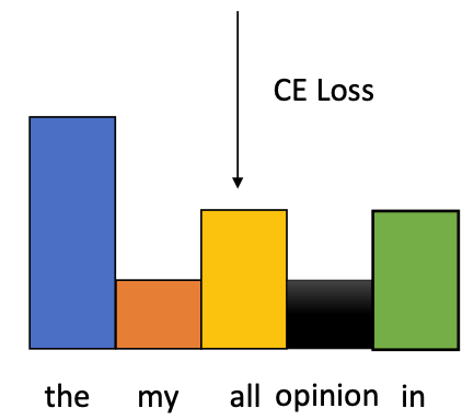
Backpropagation in the model

• Gradient of the loss function

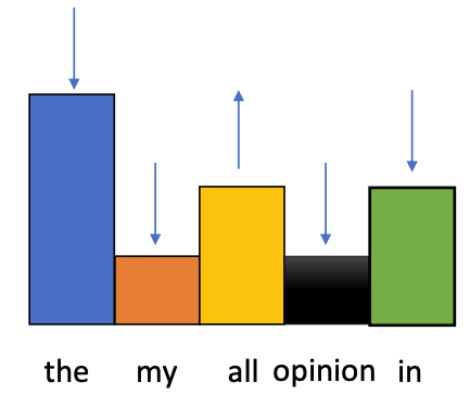
  $$ \frac{d L\_t}{d o\_t} = p\_t - y\_t $$

• $y\_t$ in Char-Language-Model is an one-hot-vector

  $\to$ The gradient is positive everywhere and negative in the label position

  $p\_{t\_i} \in (0, 1)$

  Assume the label is in the $i$-th position.

  • In non-label position:

    $$ > \forall j \neq i: \qquad y\_{t\_j} = 0 \\\\ > \Rightarrow p\_{t\_i} - y\_{t\_i} = p\_{t\_i} - 0 = p\_{t\_i} > 0 > $$

  • In label position:

    $$ > y\_{t\_i} = 1 \Rightarrow p\_{t\_i} - y\_{t\_i} = p\_{t\_i} - 1 < 0 > $$

  

• Gradient at the hidden layer:

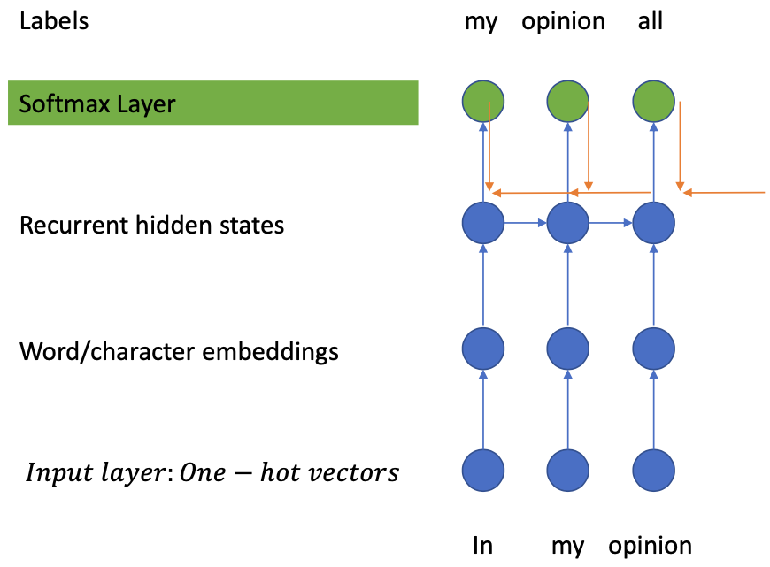  - The hidden layer $h\_t$ receives two sources of gradients: - Coming from the loss of the current state - Coming from the gradient carried over from the future - Similary the memory cell $c\_t$: - Receives the gradient from the $h\_t$ - Summing up that gradient with the gradient coming from the future

Generate a New Sequence

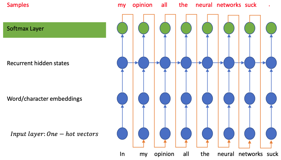
• Start from a memory state of the RNN (often initialized as zeros)

• Run the network through a seed

• Generate the probability distribution given the seed and the memory state

• “Sample” a new token from the distribution

• Use the new token as the seed and carry the new memory over to keep generating

Sequence-to-Sequence Models

💡 Main idea: from $P(W)$ to $P(W \mid C)$ with $C$ being a context

Controlling Generation with RNN

Hints:

• The generated sequence depends on

  • The first input(s)

  • The first recurrent hidden state

    

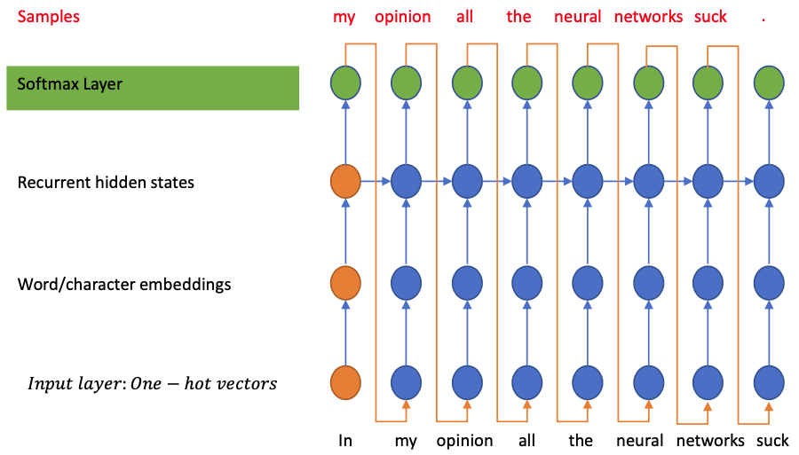
• The final hidden state of the network after rolling contains the compressed information about the sequence

  

Sequence-to-Sequence problem

• Given: sequence $X$ of variable length (source sequence)

  $$ X = (X\_1, X\_2, \dots, X\_m) $$

• Task: generate a new sequence $Y$ that has the same content

  $$ Y = (Y\_1, Y\_2, \dots, X\_n) $$

• Training:

  • Given the dataset $𝐷$ containing pairs of parallel sentences $(𝑋, 𝑌)$

  • Training objective

    $$ \log P\left(Y^{\*} \mid X^{\*}\right) \qquad \forall \left(\mathrm{Y}^{\*}, \mathrm{X}^{\*}\right) \in D $$

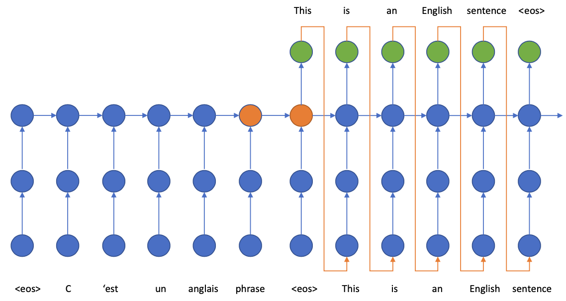
Encoder-Decoder model

Encoder

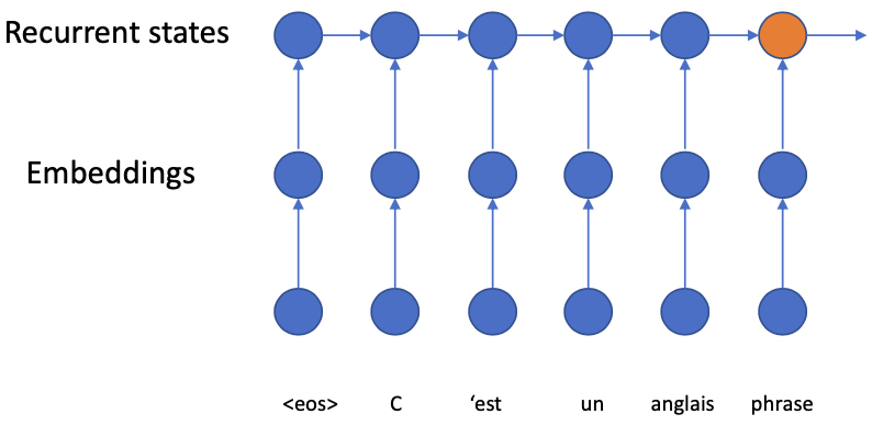
• Transforms the input into neural representation

• Input

  • Discret variables: require using embedding to be “compatible” with neural networks
  • Continuous variables: can be “raw features” of the input
    • Speech signals
    • Image pixels

• The encoder represents the $X$ part

• The generative chain does not incline any generation from the encoder

Decoder

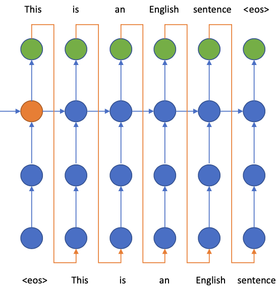
• The encoder gives the decoder a representation of the source input
• The decoder would try to “decode” the information from that representation
• Key idea: the encoder representation is the $H\_0$ of the decoder network
• The operation is identical to the character-based language model
  • Back-propagation through time provides the gradient w.r.t any hidden state
    • For the decoder: the BPTT is identical to the language model
    • For the encoder: At each step the encoder hidden state only has 1 source of gradient

Problem with Encoder-Decoder Model

The model worked well to translate short sentences. But long sentences (more than 10 words) suffered greatly 😢

🔴 Main problem:

• Long-range dependency
• Gradient starving

Funny trick Solution: Reversing the source sentence to make the sentence starting words closer. (pretty “hacky” 😈)

Observation for solving this problem

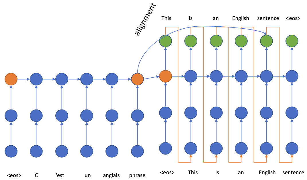
Each word in the source sentence can be aligned with some words in the target sentence. (“alignment” in Machine Translation)

We can try to establish a connection between the aligned words.

Seq2Seq with Attention

As mentioned, we want to find the alignment between decoder-encoder. However, Our decoder only looks at the final and compressed encoder state to find the information.

Therefore we have to modify the decoder to do better! 💪

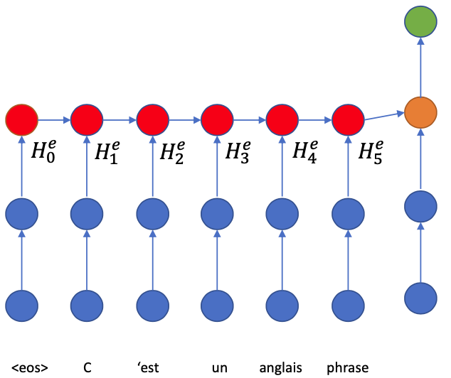
1. Run the encoder LSTM through the input sentence (Read the sentence and encode it into states
2. The LSTM operation gives us some assumption about $H\_j^e$
3. The state $H\_j^e$ contains information about
   • the word $W\_j$ (because of input gate)
   • some information about the surrounding (because of memory))

Now we start generating the translation with the decoder.

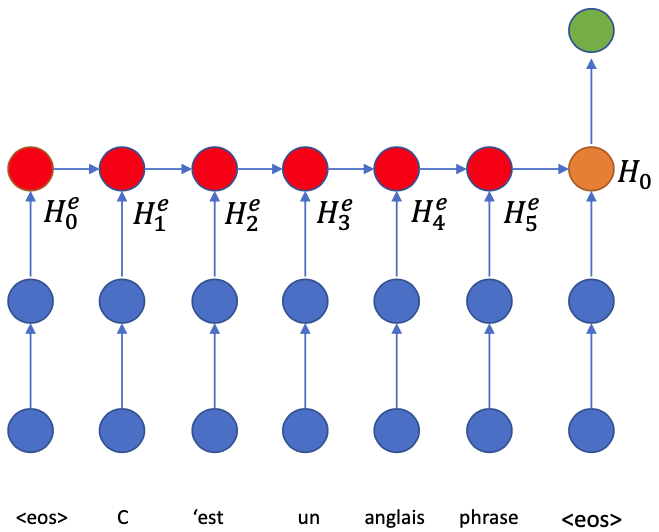
4. The LSTM consumes the EOS token (always) and the hidden states copied over to get the first hidden state $H\_0$

5. From $H\_0$ we have to generate the first word, and we need to look back to the encoder.

   • Here we ask the question:

     “Which word is responsible to generate the first word?”

   • However, it’s not easy to answer this question

     • First we don’t know 😭
     • Second there might be more than one relevant word (like when we translate phrases or compound words) 🤪

The best way to find out is: to check all of the words! 💪

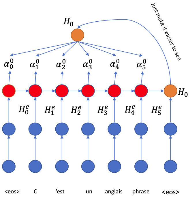
6. $H\_0$ has to connect all $H\_i^e$ in the encoder side for querying

7. Each “connection” will return a score $\alpha\_i$ indicating how relevant $H\_i^e$ is to generate the translation from $H\_0$

   • Generate $\alpha_i^0$

     1. A feed forward neural network with nonlinearity
     $$ \alpha\_{i}^{0}=\mathrm{W}\_{2} \cdot \tanh \left(\mathrm{W}\_{1} \cdot\left[\mathrm{H}_{0}, \mathrm{H}\_{1}^{\mathrm{e}}\right]+b\_{1}\right) $$
     2. Use Softmax to get probabilities $$ \alpha \leftarrow \operatorname{softmax}(\alpha) $$

8. The higher $\alpha\_i$ is, the more relevant the state $H\_i^e$ is

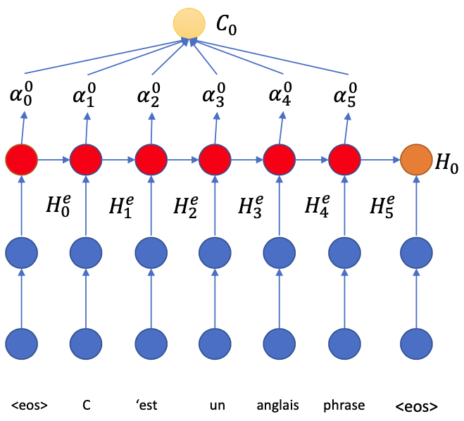
After $H\_0$ asks “Everyone” in the encoder, it needs to sum up the information

$$ C\_0 = \sum\_i \alpha\_i^0 H\_i^e $$

($C\_0$ is the summarization of the information in the encoder that is the most relevant to $H\_0$ to generate the first word in the decoder)

9. Now we can answer the question “Which word is responsible to generate the first word?”

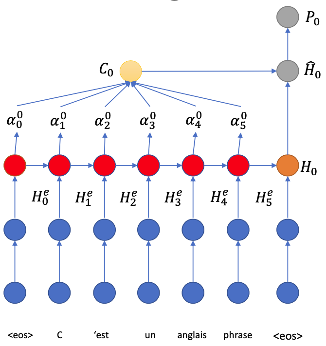
The answer is: the words with highest $\alpha$ coefficients

• Combine $H\_0$ with $C\_0$
• Generate the softmax output $P\_0$ from $\hat{H}\_0$
• Go to the next step

In general, at time step $t$:

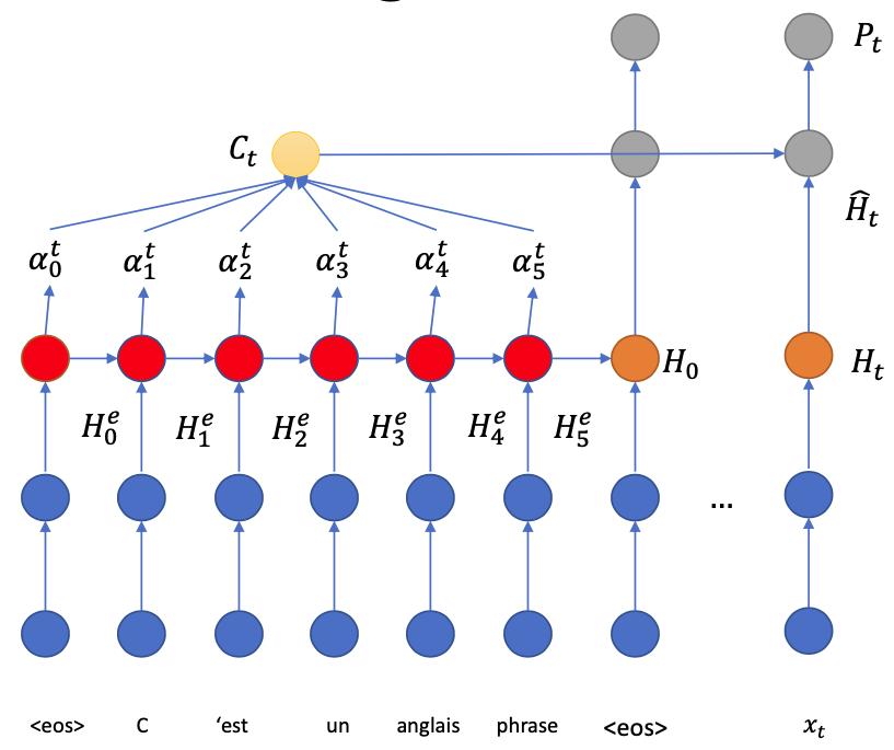
• Decoder LSTM generates the hidden state $H\_t$ from the memory $H\_{t-1}$

• $H\_t$ “pays attention” to the encoder states to know which source information is relevant

• Generate $\alpha\_i^t$ from each $H\_i^e$

• Weighted sum for “context vector” $C\_t$

• Combine $C\_t$ and $H\_t$ then generates $P\_t$ for output distribution

  • Use a feed-forward neural network

    $$ \hat{H}\_t = \operatorname{tanh}(W\cdot [C\_t, H\_t]) $$

  • Or use a RNN

    $$ \hat{H}\_t = \operatorname{RNN}(C\_t, H\_t) $$

Training

• Very similar to basic Encoder-Decoder
• Since the scoring neural network is continuous, we can use backpropagation
• No loner gradient starving on the encoder side

Pratical Suggestions for Training

• Loss is too high and generation is garbarge

  • Try to match your implementation with the LSTM equations
  • Check the gradients by gradcheck
  • Note that the gradcheck can still return some weights not passing the relative error check, but acceptable if only several (1 or 2% of the weights) cannot pass

• Loss looks decreasing and the generated text looks correct but not readable

  • In the sampling process, you can encourage the model to generate with higher certainty by using “argmax” (taking the char with highest probability)
  • But “always using argmax” will look terrible
  • A mixture of argmax and sampling can be used to ensure spelling correctness and exploration

• Large network size is normally needed for character based models