Auto Encoder
Supervised vs. Unsupervised Learning
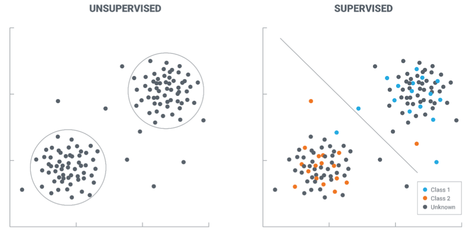
Supervised vs. unsupervised
- Supervised learning
- Given data $(X, Y)$
- Estimate the posterior $P(Y|X)$
- Unsupervised learning
- Concern with the structure (unseen) of the data
- Try to estimate (implicitly or explicitly) the data distribution $P(X)$
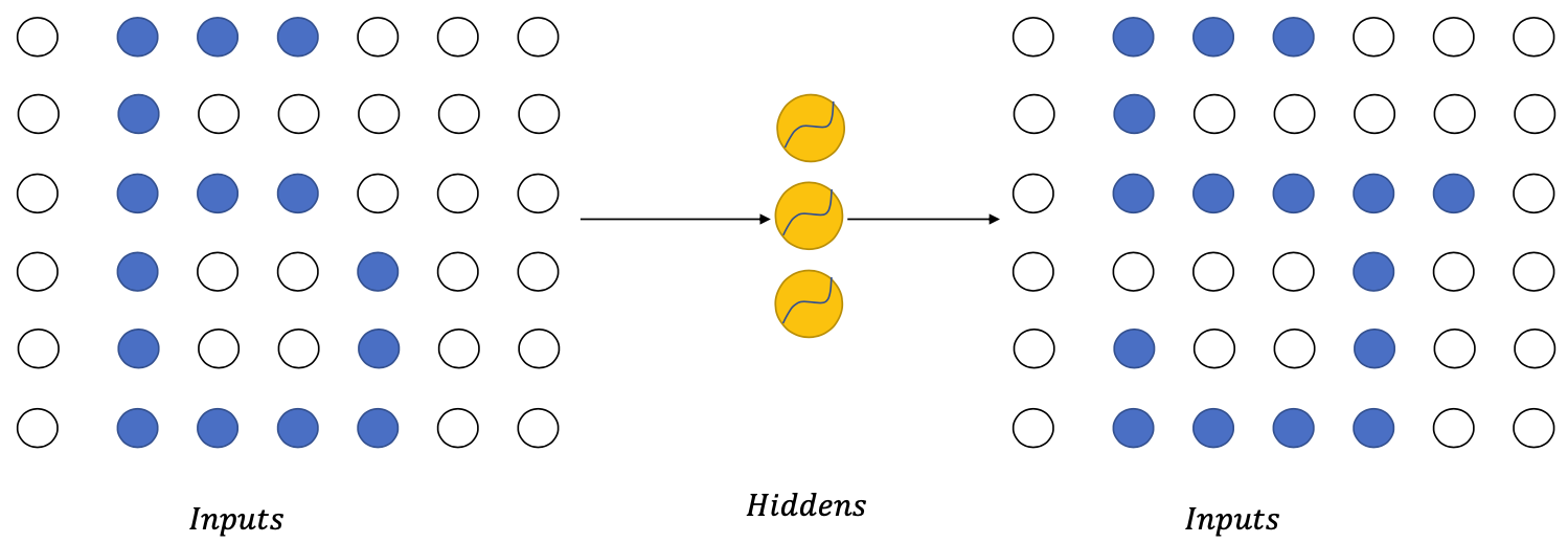
Auto-Encoder structure
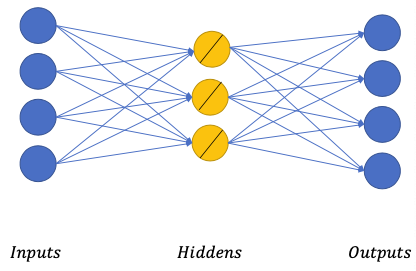
In supervised learning, the hidden layers encapsulate the features useful for classification. Even there are no labels or no output layer, it is still possible to learn features in the hidden layer! 💪
Linear auto-encoder
 $$
\begin{array}{l}
H=W\_{I} I+b\_{I} \\\\
\tilde{I}=W\_{O} H+b\_{O}
\end{array}
$$
$$
\begin{array}{l}
H=W\_{I} I+b\_{I} \\\\
\tilde{I}=W\_{O} H+b\_{O}
\end{array}
$$- Similar to linear compression method (such as PCA)
- Trying to find linear surfaces that most data points can lie on
- Not very useful for complicated data 🤪
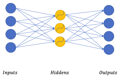
Non-linear auto-encoder
 $$
\begin{array}{l}
H=f(W\_{I} I+b\_{I}) \\\\
\tilde{I}=W\_{O} H+b\_{O}
\end{array}
$$
$$
\begin{array}{l}
H=f(W\_{I} I+b\_{I}) \\\\
\tilde{I}=W\_{O} H+b\_{O}
\end{array}
$$When $D\_H > D\_I$, the activation function also prevents the network to simply copy over the data
Goal: find optimized weights to minimize
$$ L=\frac{1}{2}(\tilde{I}-\mathrm{I})^{2} $$- Optimized with Stochastic Gradient Descent (SGD)
- Gradients computed with Backpropagation
General auto-encoder structure
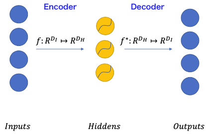
2 components in general
- Encoder: maps input $I$ to hidden $H$
- Decoder: reconstructs $\tilde{I}$ from $H$
($f$ and $f^*$ depend on input data type)
Encoder and Decoder often have similar/reversed architectures
Why Auto-Encoders?
With auto-encoders we can do
- Compression & Reconstruction
- MLP training assistance
- Feature learning
- Representation learning
- Sampling different variations of the inputs
There’re many types and variations of auto-encoders
Different architectures for different data types
Different loss functions for different learning purposes
Compression and Reconstruction
$D\_H < D\_I$
- For example a flattened image: $D\_I = 1920 \times 1080 \times 3$
- Common hidden layer sizes: $512$ or $1024$
$\to$ Sending $H$ takes less bandwidth then $I$
Sender uses $W\_I$ and $b\_I$ to compress $I$ into $H$
Receiver uses $W\_O$ and $b\_O$ to reconstruct $\tilde{I}$
With corrupted inputs
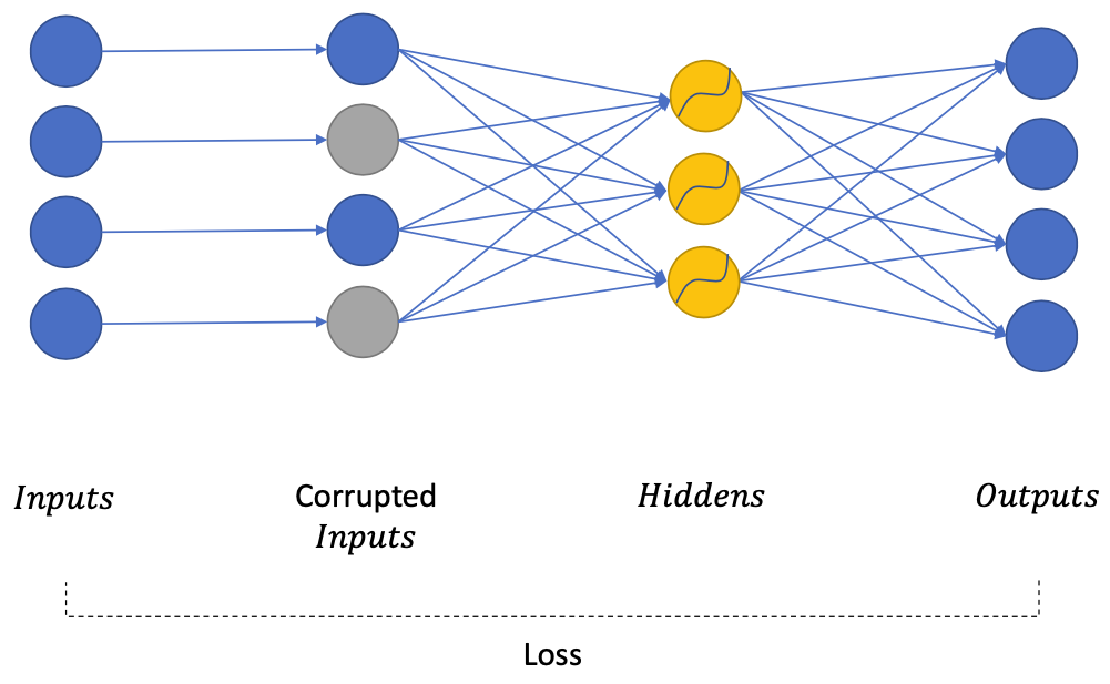
Deliberately corrupt inputs
Train auto-encoders to regenerate the inputs before corruption
$D\_H < D\_I$ NOT required (no risk of learning an identity function)
Benefit from a network with large capacity
Different ways of corruption
- Images
- Adding noise filters
- downscaling
- shifting
- …
- Speech
- simulating background noise
- Creating high-articulation effect
- …
- Text: masking words/characters
- Images
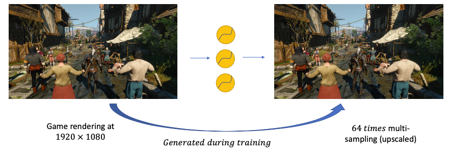
Application
Deep Learning super sampling
- use neural auto-encoders to generate HD frames from SD frames
Denoising Speech from Microphones
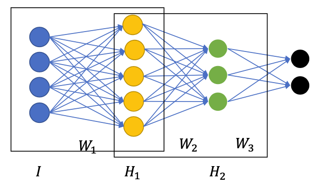
Unsupervised Pretraining
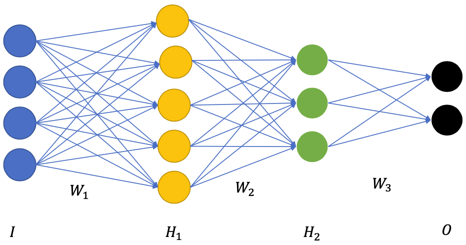
Normal training regime
- Initialize the networks with random $W\_1, W\_2, W\_3$
- Forward pass to compute output $O$
- Get the loss function $L(O, Y)$
- Backward pass and update weights to minimize $L$
Pretraining regime
- Find a way to have $W\_1, W\_2, W\_3$ pretrained 💪
- They are used to optimize auxiliary functions before training
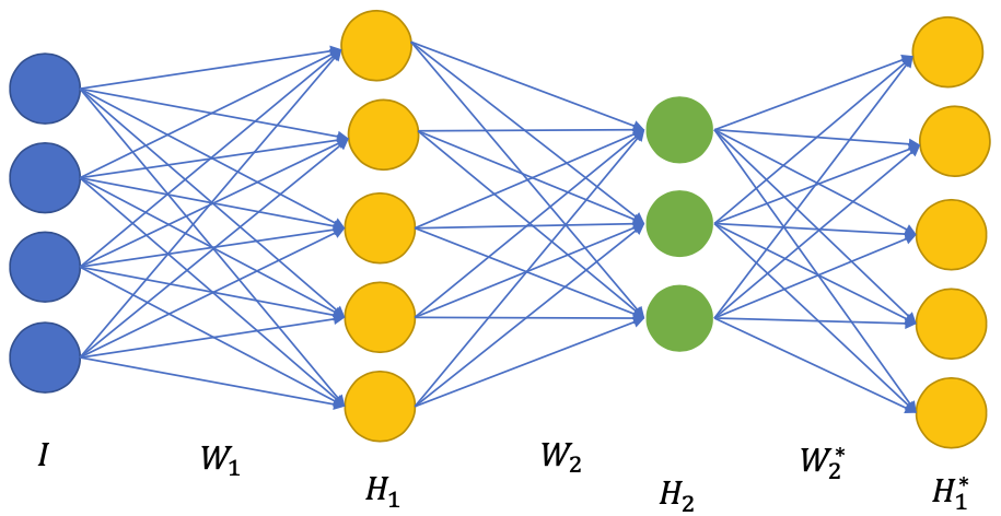
Layer-wise pretraining
Pretraining first layer
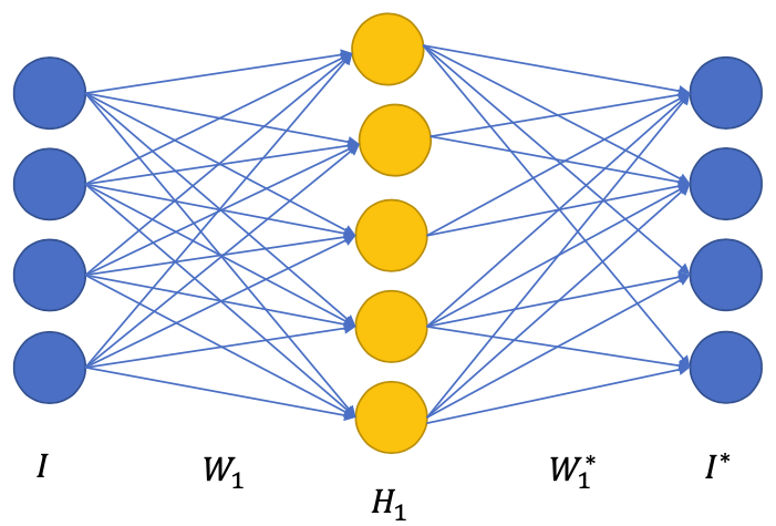
Initialize $W\_1$ to encode, $W\_1^*$ to decode
Forward pass
$I \to H\_1 \to I^*$
Reconstruction loss:
$$ L = \frac{1}{2}(I^* - I)^2 $$
Backward pass
- Compute gradients $\frac{\delta L}{\delta W_{1}}$ and $\frac{\delta L}{\delta W_{1}^*}$
Update $W\_1$, $W\_1^*$ with SGD
Repeat 1 to 4 until convergence
Pretraining next layers
- Use $W\_1$ from previous pretraining
Initialize $W\_2$ to encode, $W\_2^*$ to decode
Forward pass
$I \to H\_1 \to H\_2 \to I^*$
Reconstruction loss:
$$ L = \frac{1}{2}(H\_1^* - H\_1)^2 $$
Backward pass
- Compute gradients $\frac{\delta L}{\delta W_{2}}$ and $\frac{\delta L}{\delta W_{2}^*}$
Update $W\_2$, $W\_2^*$ with SGD and keep $W\_1$ the same
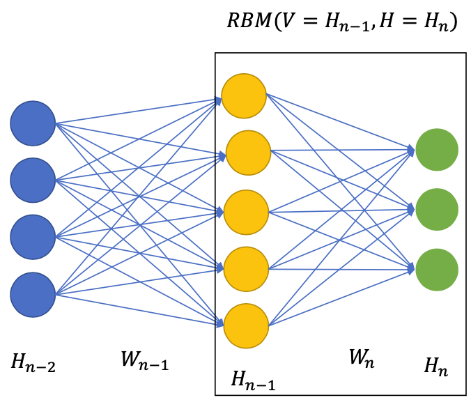
Hidden layers pretraining in general
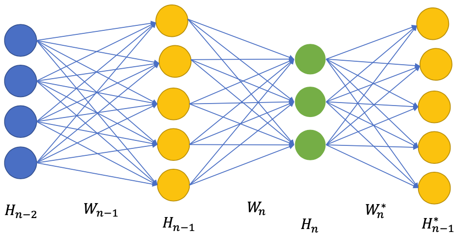
- Each layer $H\_n$ is pretrained as an AE to reconstruct the input of that layer (i.e $H\_{n-1}$)
- The backward pass is stopped at the input to prevent changing previous weights $W\_1, \dots, W\_{n-1}$ and ONLY update $W\_n, W\_n^*$
- Complexity of each AE increases over depth (since the forward pass requires all previously pretrained layers)
Finetuning
- Start the networks with pretrained $W\_1, W\_2, W\_3$
- Go back to supervised training:
- Forward pass to compute output $O$
- Get the loss function $L(O, Y)$
- Backward pass and update weights to minimize $L$
This process is called finetuning because the weights are NOT randomly initialized, but carried over from an external process
What does “unsupervised pretraining” help?
According to Why Does Unsupervised Pre-training Help Deep Learning?
- Pretraining helps to make networks with 5 hidden layers converge
- Lower classification error rate
- Create a better starting point for the non-convex optimization process
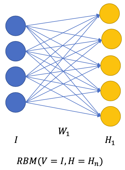
Restricted Boltzmann Machine

Structure
- Visible units (Input data points $I$)
- Hidden units ($H$)
Given input $V$, we can generate the probabilities of hidden units being On(1)/Off (0)
$$ p\left(h\_{j}=1 \mid V\right)=\sigma\left(b\_{j}+\sum\_{i=1}^{m} W\_{i j} v\_{i}\right) $$Given the hidden units, we can generate the probabilities of visible units being On/Off
$$ p\left(v\_{i} \mid H\right)=\sigma\left(b\_{i}+\sum\_{j=1}^{F} W\_{i j} h\_{j}\right) $$Energy function of a visible-hidden system
$$ E(V, H)=-\sum\_{i=1}^{m} \sum\_{j=1}^{F} W\_{i j} h\_{j} v\_{i}-\sum\_{i=1}^{m} v\_{i} a\_{i}-\sum\_{j=1}^{F} h\_{j} b\_{j} $$- Train the network to minimize the energy function
- Use Contrastive Divergence algorithm
Layer-wise pretraining with RBM
Finetuning RBM: Deep Belief Network
- The end result is called a Deep Belief Network
- Use pretrained $W\_1, W\_2, W\_3$ to convert the network into a typical MLP
- Go back to supervised training:
- Forward pass to compute output $O$
- Get the loss function $L(O, Y)$
- Backward pass and update weights to minimize $L$
RBM Pretraining application in Speech
Speech Recognition = Looking for the most probable transcription given an audio
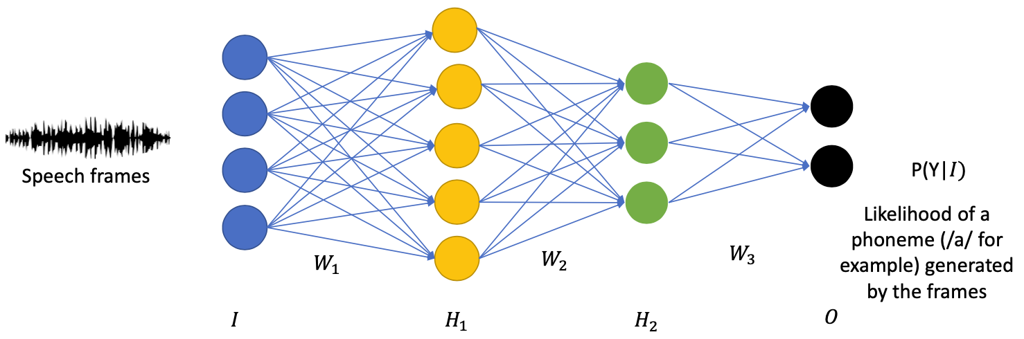
💡 We can use (deep) neural networks to replace the non-neural generative models (Gaussian Mixture Models) in the Acoustic Models
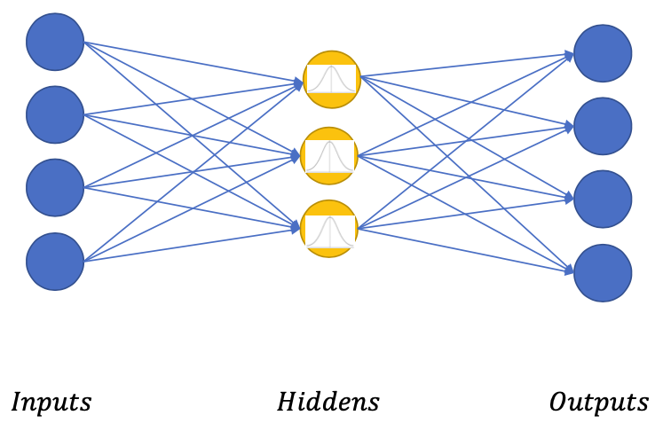
Variational Auto-Encoder
💡 Main idea:Enforcing the hidden units to follow an Unit Gaussian Distribution (or a known distribution)
- In AE we didn’t know the “distribution” of the (hidden) code
- Knowing the distribution in advance will make sampling easier
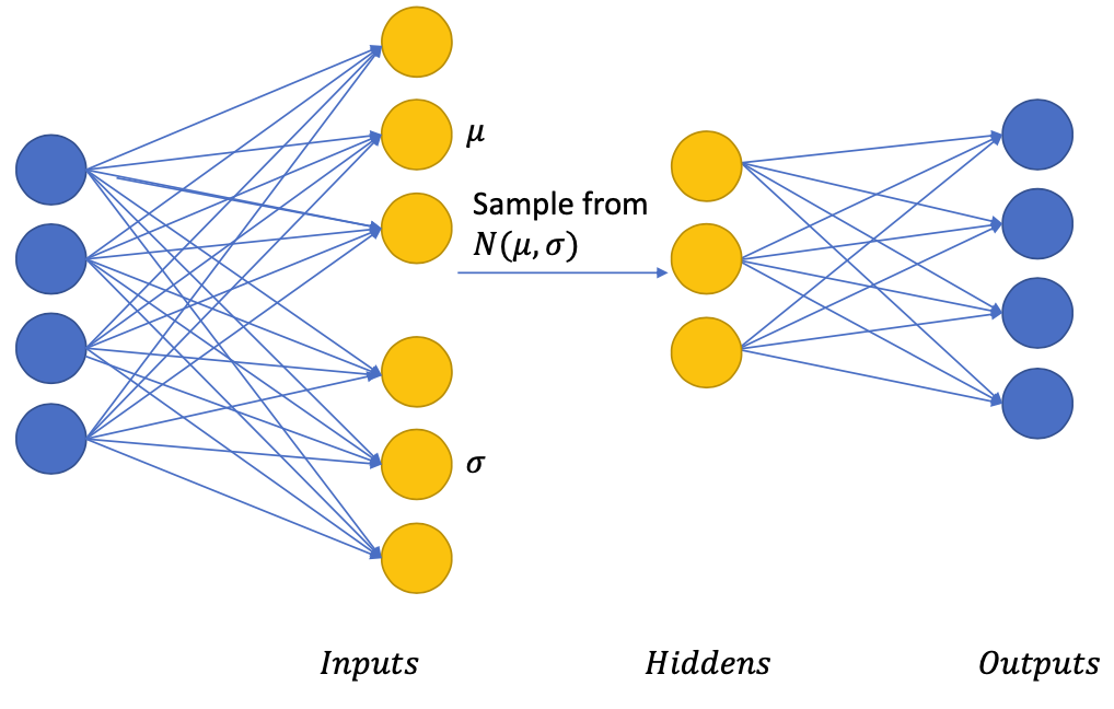
Get the Gaussian restriction
- Each Gaussian is represented by Mean $𝜇$ and Variance $𝜎$
Why do we sample?
- The hidden layers’ neurons are then “arranged” in the gaussian distribution
We wanted to enforce the hidden layers to follow a known distribution, for example $𝑁(0, 𝐼)$, so we can add a loss function to do so:
$$ L=\frac{1}{2}(O-I)^{2}+\mathrm{KL}(\mathrm{N}(0, I), \mathrm{N}(\mu, \sigma)) $$Variational methods allow us to take a sample of the distribution being estimated, then get a “noisy” gradient for SGD
Convergence can be achieved in practice
Structure Prediction
Beyond auto-encoder
- Auto-Encoder
- Given the object: reconstruct the object
- $P(X)$ is (implicitly) estimated via reconstructing the inputs
- Structure prediction
- Given a part of the object: predict the remaining
- $P(X)$ is estimated by factorizing the inputs
- Auto-Encoder
Example
Pixel Models
Assumption (biased): The pixels are generated from left to right, from top to bottom.
(I.e. the content of each pixel depends only on the pixels on its left, and its top rows, like image)
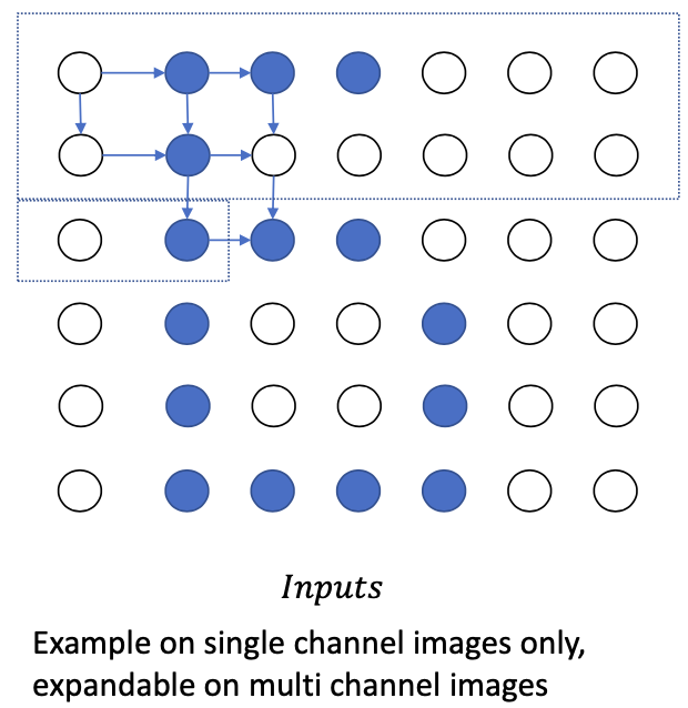
We can estimate a probabilistic function to learn how to generate pixels
- Image $X = \\{x\_1, x\_2, \dots, x\_n\\}$ with $n$ pixels $$ P(X)=\prod\_{i=1}^{n} p\left(x\_{i} \mid x\_{1}, \ldots x\_{i-1}\right) $$
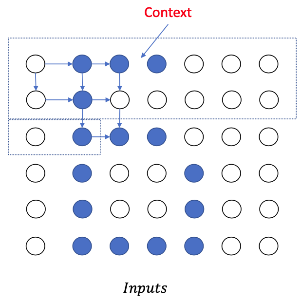
Closer look:
- But this is quite difficult
- The number of input pixels is a variable
- There are many pixels in an image
- We can model such context dependency using many types of neural networks:
Recurrentneuralnetworks
Convolutional neural networks
Transformers/Self-attentionNN
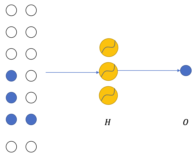
(Neural) Language Models
A common model/application in natural language processing and generation (E.g. chatbots, translation, question answering)
Similar to the pixel models, we can assume the words are generated from left to right
$$ P( \text{the end of our life} )=P( \text{the} ) \times P( \text{end} \mid {the} ) \times P(\text{of} \mid \text{the end} ) \times P( \text{our} \mid \text{the end of} ) \times P(\text{life} \mid \text{the end of our}) $$Each term can be estimated using neural networks under the form $P(x|context)$ with context being a series of words
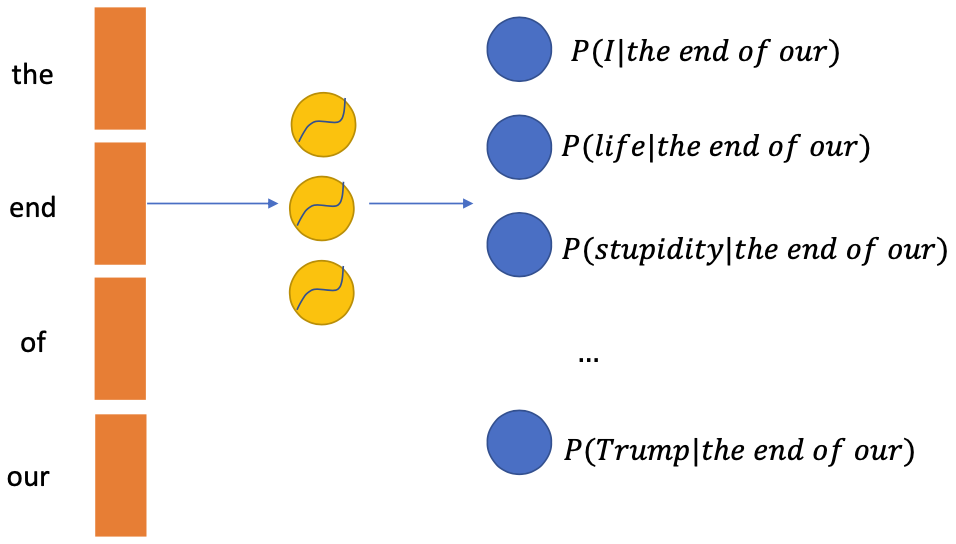
- Input: context
- Output: classification with $V$ classes (the vocabulary size)
- Most classes will have near 0 probabilities given the context
Summary
- Structure prediction is
- An explicit and flexible method to deal with estimating the likelihood of data that can be factorized (with bias)
- Motivation to develop a lot of flexible techniques
- Such as sequence to sequence models, attention models
- The bias is often the weakness 🤪