Bolzmann Machine
Boltzmann Machine
- Stochastic recurrent neural network
- Introduced by Hinton and Sejnowski
- Learn internal representations
- Problem: unconstrained connectivity
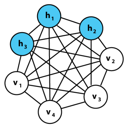
Representation
Model can be represented by Graph:
Undirected graph
Nodes: States
States
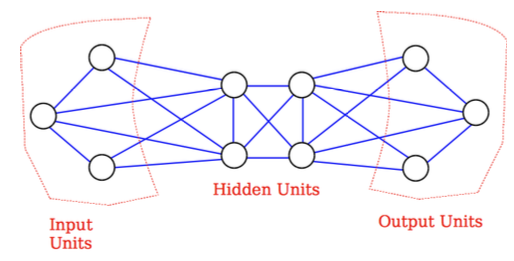
Types:
- Visible states
- Represent observed data
- Can be input/output data
- Hidden states
- Latent variable we want to learn
- Bias states
- Always one to encode the bias
Binary states
- unit value $\in \\{0, 1\\}$
Stochastic
Decision of whether state is active or not is stochastically
Depend on the input
$$ z\_{i}=b\_{i}+\sum\_{j} s\_{j} w\_{i j} $$- $b\_i$: Bias
- $S\_j$: State $j$
- $w\_{ij}$: Weight between state $j$ and state $i$
Connections
Graph can be fully connected (no restrictions)
Unidircted:
$$ w\_{ij} = w\_{ji} $$No self connections:
$$ w\_{ii} = 0 $$
Energy
Energy of the network
$$ \begin{aligned} E &= -S^TWS - b^TS \\\\ &= -\sum\_{iUpdating the nodes
decrease the Energy of the network in average
reach Local Minimum (Equilibrium)
Stochastic process will avoid local minima
$$ \begin{array}{c} p\left(s\_{i}=1\right)=\frac{1}{1+e^{-z\_{i}}} \\\\ z\_{i}=\Delta E\_{i}=E\_{i=0}-E\_{i=1} \end{array} $$
Simulated Annealing
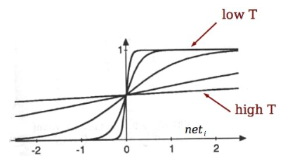
Use Temperature to allow for more changes in the beginning
Start with high temperature
“anneal” by slowing lowering T
Can escape from local minima 👏
Search Problem
Input is set and fixed (clamped)
Annealing is done
Answer is presented at the output
Hidden units add extra representational power
Learning problem
Situations
- Present data vectors to the network
Problem
- Learn weights that generate these data with high probability
Approach
- Perform small updates on the weights
- Each time perform search problem
Pros & Cons
✅ Pros
- Boltzmann machine with enough hidden units can compute any function
⛔️ Cons
- Training is very slow and computational expensive 😢
Restricted Boltzmann Machine
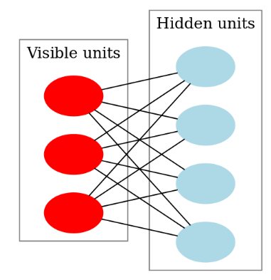
Boltzmann machine with restriction
Graph must be bipartite
Set of visible units
Set of hidden units
✅ Advantage
- No connection between hidden units
- Efficient training
Energy
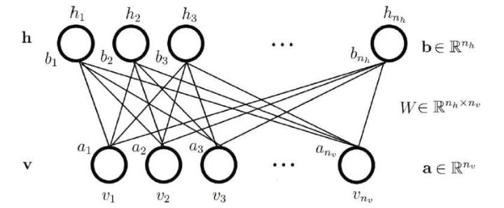
Energy:
$$ \begin{aligned} E(v, h) &= -a^{\mathrm{T}} v-b^{\mathrm{T}} h-v^{\mathrm{T}} W h \\\\ &= -\sum\_{i} a\_{i} v\_{i}-\sum\_{j} b\_{j} h\_{j}-\sum_{i} \sum_{j} v_{i} w_{i j} h_{j} \end{aligned} $$Probability of hidden unit:
$$ p\left(h\_{j}=1 \mid V\right)=\sigma\left(b\_{j}+\sum\_{i=1}^{m} W\_{i j} v\_{i}\right) $$Probability of input vector:
$$ p\left(v\_{i} \mid H\right)=\sigma\left(a\_{i}+\sum\_{j=1}^{F} W\_{i j} h\_{j}\right) $$$$ > \sigma(x)=\frac{1}{1+e^{-x}} > $$
Free Energy:
$$ \begin{array}{l} e^{-F(V)}=\sum\_{j=1}^{F} e^{-E(v, h)} \\\\ F(v)=-\sum\_{i=1}^{m} v\_{i} a\_{i}-\sum_{j=1}^{F} \log \left(1+e^{z_{j}}\right) \\\\ z_{j}=b\_{j}+\sum\_{i=1}^{m} W\_{i j} v\_{i} \end{array} $$