SVM: Basics
🎯 Goal of SVM
To find the optimal separating hyperplane which maximizes the margin of the training data
- it correctly classifies the training data
- it is the one which will generalize better with unseen data (as far as possible from data points from each category)
SVM math formulation
Assuming data is linear separable
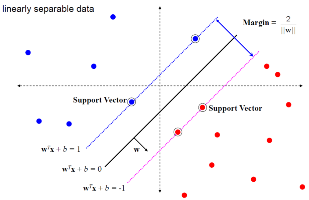
Decision boundary: Hyperplane $\mathbf{w}^{T} \mathbf{x}+b=0$
Support Vectors: Data points closes to the decision boundary (Other examples can be ignored)
- Positive support vectors: $\mathbf{w}^{T} \mathbf{x}_{+}+b=+1$
- negative support vectors: $\mathbf{w}^{T} \mathbf{x}_{-}+b=-1$
Why do we use 1 and -1 as class labels?
- This makes the math manageable, because -1 and 1 are only different by the sign. We can write a single equation to describe the margin or how close a data point is to our separating hyperplane and not have to worry if the data is in the -1 or +1 class.
- If a point is far away from the separating plane on the positive side, then $w^Tx+b$ will be a large positive number, and $label*(w^Tx+b)$ will give us a large number. If it’s far from the negative side and has a negative label, $label*(w^Tx+b)$ will also give us a large positive number.
Margin $\rho$ : distance between the support vectors and the decision boundary and should be maximized
$$ \rho = \frac{\mathbf{w}^{T} \mathbf{x}\_{+}+b}{\|\mathbf{w}\|}-\frac{\mathbf{w}^{T} \mathbf{x}\_{-}+b}{\|\mathbf{w}\|}=\frac{2}{\|\mathbf{w}\|} $$
SVM optimization problem
Requirement:
- Maximal margin
- Correct classification
Based on these requirements, we have:
Reformulation:
$$ \begin{aligned} \underset{\mathbf{w}}{\operatorname{argmin}} \quad &\\|\mathbf{w}\\|^{2} \\\\ \text {s.t.} \quad & y_{i}\left(\mathbf{w}^{T} \mathbf{x}\_{i}+b\right) \geq 1 \end{aligned} $$This is the hard margin SVM.
Soft margin SVM
💡 Idea
“Allow the classifier to make some mistakes” (Soft margin)
➡️ Trade-off between margin and classification accuracy
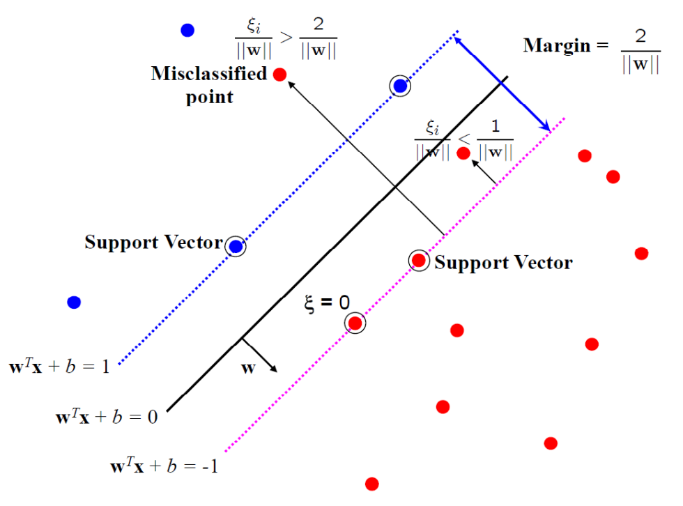
Slack-variables: ${\color {blue}{\xi_{i}}} \geq 0$
💡Allows violating the margin conditions
$$ y_{i}\left(\mathbf{w}^{T} \mathbf{x}_{i}+b\right) \geq 1- \color{blue}{\xi_{i}} $$- $0 \leq \xi\_{i} \leq 1$ : sample is between margin and decision boundary (margin violation)
- $\xi\_{i} \geq 1$ : sample is on the wrong side of the decision boundary (misclassified)
Soft Max-Margin
Optimization problem
$$ \begin{array}{lll} \underset{\mathbf{w}}{\operatorname{argmin}} \quad &\|\mathbf{w}\|^{2} + \color{blue}{C \sum_i^N \xi_i} \qquad \qquad & \text{(Punish large slack variables)}\\\\ \text { s.t. } \quad & y_{i}\left(\mathbf{w}^{T} \mathbf{x}_{i}+b\right) \geq 1 -\color{blue}{\xi_i}, \quad \xi_i \geq 0 \qquad \qquad & \text{(Condition for soft-margin)}\end{array} $$- $C$ : regularization parameter, determines how important $\xi$ should be
- Small $C$: Constraints have little influence ➡️ large margin
- Large $C$: Constraints have large influence ➡️ small margin
- $C$ infinite: Constraints are enforced ➡️ hard margin
Soft SVM Optimization
Reformulate into an unconstrained optimization problem
- Rewrite constraints: $\xi_{i} \geq 1-y_{i}\left(\mathbf{w}^{T} \mathbf{x}_{i}+b\right)=1-y_{i} f\left(\boldsymbol{x}_{i}\right)$
- Together with $\xi_{i} \geq 0 \Rightarrow \xi_{i}=\max \left(0,1-y_{i} f\left(\boldsymbol{x}_{i}\right)\right)$
Unconstrained optimization (over $\mathbf{w}$):
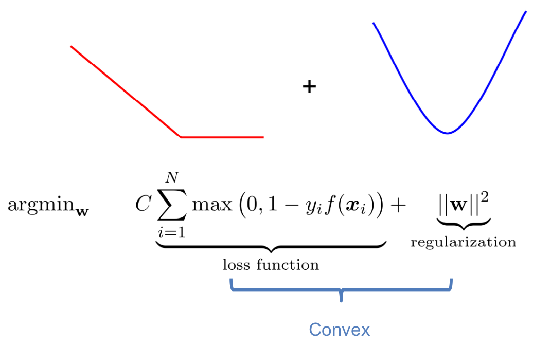
$$ \underset{{\mathbf{w}}}{\operatorname{argmin}} \underbrace{\|\mathbf{w}\|^{2}}\_{\text {regularization }}+C \underbrace{\sum_{i=1}^{N} \max \left(0,1-y\_{i} f\left(\boldsymbol{x}\_{i}\right)\right)}_{\text {loss function }} $$Points are in 3 categories:
$y\_{i} f\left(\boldsymbol{x}\_{i}\right) > 1$ : Point outside margin, no contribution to loss
$y\_{i} f\left(\boldsymbol{x}\_{i}\right) = 1$: Point is on the margin, no contribution to loss as in hard margin
$y\_{i} f\left(\boldsymbol{x}\_{i}\right) < 1$: Point violates the margin, contributes to loss
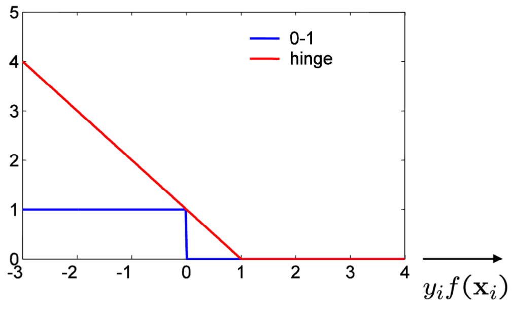
Loss function
SVMs uses “hinge” loss (approximation of 0-1 loss)
For an intended output $t=\pm 1$ and a classifier score $y$, the hinge loss of the prediction $y$ is defined as
$$ > \ell(y)=\max (0,1-t \cdot y) > $$Note that $y$ should be the “raw” output of the classifier’s decision function, not the predicted class label. For instance, in linear SVMs, $y = \mathbf{w}\cdot \mathbf{x}+ b$, where $(\mathbf{w},b)$ are the parameters of the hyperplane and $mathbf{x}$ is the input variable(s).
The loss function of SVM is convex:
I.e.,
- There is only one minimum
- We can find it with gradient descent
- However: Hinge loss is not differentiable! 🤪
Sub-gradients
For convex function $f: \mathbb{R}^d \to \mathbb{R}$ :
$$ f(\boldsymbol{z}) \geq f(\boldsymbol{x})+\nabla f(\boldsymbol{x})^{T}(\boldsymbol{z}-\boldsymbol{x}) $$(Linear approximation underestimates function)
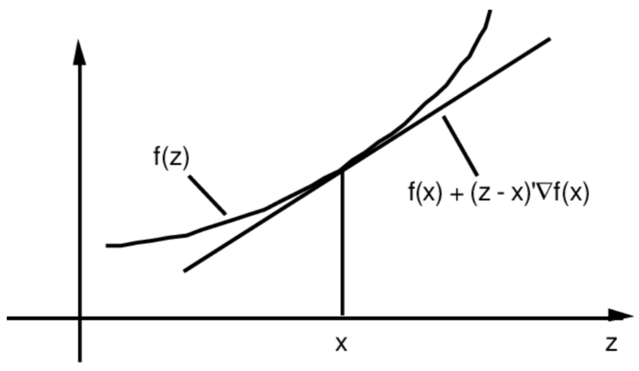
A subgradient of a convex function $f$ at point $\boldsymbol{x}$ is any $\boldsymbol{g}$ such that
$$ f(\boldsymbol{z}) \geq f(\boldsymbol{x})+\nabla \mathbf{g}^{T}(\boldsymbol{z}-\boldsymbol{x}) $$- Always exists (even $f$ is not differentiable)
- If $f$ is differentiable at $\boldsymbol{x}$, then: $\boldsymbol{g}=\nabla f(\boldsymbol{x})$
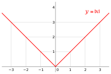
Example
$f(x)=|x|$
- $x \neq 0$ : unique sub-gradient is $g= \operatorname{sign}(x)$
- $x =0$ : $g \in [-1, 1]$
Sub-gradient Method
Sub-gradient Descent
- Given convex $f$, not necessarily differentiable
- Initialize $\boldsymbol{x}_0$
- Repeat: $\boldsymbol{x}\_{t+1}=\boldsymbol{x}\_{t}+\eta \boldsymbol{g}$, where $\boldsymbol{g}$ is any sub-gradient of $f$ at point $\boldsymbol{x}_{t}$
‼️ Notes:
- Sub-gradients do not necessarily decrease $f$ at every step (no real descent method)
- Need to keep track of the best iterate $\boldsymbol{x}^*$
Sub-gradients for hinge loss
$$ \mathcal{L}\left(\mathbf{x}\_{i}, y\_{i} ; \mathbf{w}\right)=\max \left(0,1-y\_{i} f\left(\mathbf{x}\_{i}\right)\right) \quad f\left(\mathbf{x}\_{i}\right)=\mathbf{w}^{\top} \mathbf{x}\_{i}+b $$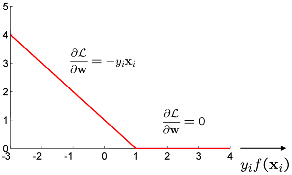
Sub-gradient descent for SVMs
Recall the Unconstrained optimization for SVMs:
$$ \underset{{\mathbf{w}}}{\operatorname{argmin}} \quad C \underbrace{\sum\_{i=1}^{N} \max \left(0,1-y_{i} f\left(\boldsymbol{x}\_{i}\right)\right)}\_{\text {loss function }} + \underbrace{\|\mathbf{w}\|^{2}}\_{\text {regularization }} $$At each iteration, pick random training sample $(\boldsymbol{x}_i, y_i)$
If $y_{i} f\left(\boldsymbol{x}_{i}\right)<1$:
$$ \boldsymbol{w}{t+1}=\boldsymbol{w}{t}-\eta\left(2 \boldsymbol{w}{t}-C y{i} \boldsymbol{x}_{i}\right) $$Otherwise:
$$ \quad \boldsymbol{w}\_{t+1}=\boldsymbol{w}\_{t}-\eta 2 \boldsymbol{w}\_{t} $$
Application of SVMs
- Pedestrian Tracking
- text (and hypertext) categorization
- image classification
- bioinformatics (Protein classification, cancer classification)
- hand-written character recognition
Yet, in the last 5-8 years, neural networks have outperformed SVMs on most applications.🤪☹️😭