Polynomial Regression (Generalized linear regression models)

💡Idea

Use a linear model to fit nonlinear data: add powers of each feature as new features, then train a linear model on this extended set of features.

Generalize Linear Regression to Polynomial Regression

In Linear Regression $f$ is modelled as linear in $\boldsymbol{x}$ and $\boldsymbol{w}$

$f(x) = \hat{\boldsymbol{x}}^T \boldsymbol{w}$

Rewrite it more generally:

$f(x) = \phi(\boldsymbol{x})^T \boldsymbol{w}$

• $\phi(\boldsymbol{x})$: vector valued funtion of the input vector $\boldsymbol{x}$ (also called “linear basis function models”)
  • $\phi_i(\boldsymbol{x})$: basis functions

In principle, this allows us to learn any non-linear function, if we know suitable basis functions (which is typically not the case 🤪).

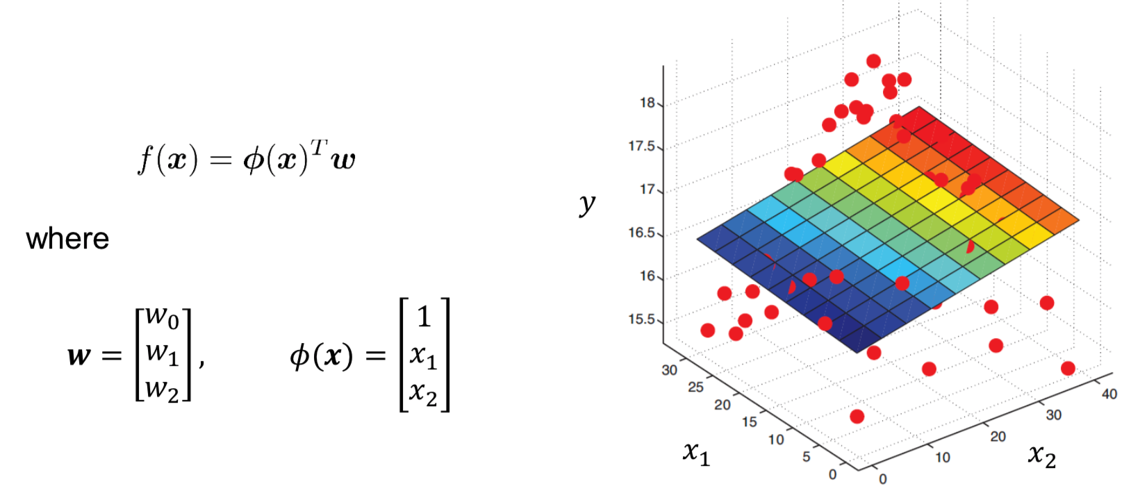
Example 1

$\boldsymbol{x}=\left[\begin{array}{c}{x_1 \\ x_2}\end{array}\right] \in \mathbb{R}^{2}$

$\phi: \mathbb{R}^2 \to \mathbb{R}^3, \left[\begin{array}{c}{x_1 \\ x_2}\end{array}\right] \mapsto \left[\begin{array}{c}{1 \\ x_1 \\ x_2}\end{array}\right]\qquad$(I.e.: $\phi_1(\boldsymbol{x}) = 1, \phi_2(\boldsymbol{x}) = x_1, \phi_3(\boldsymbol{x}) = x_2$)

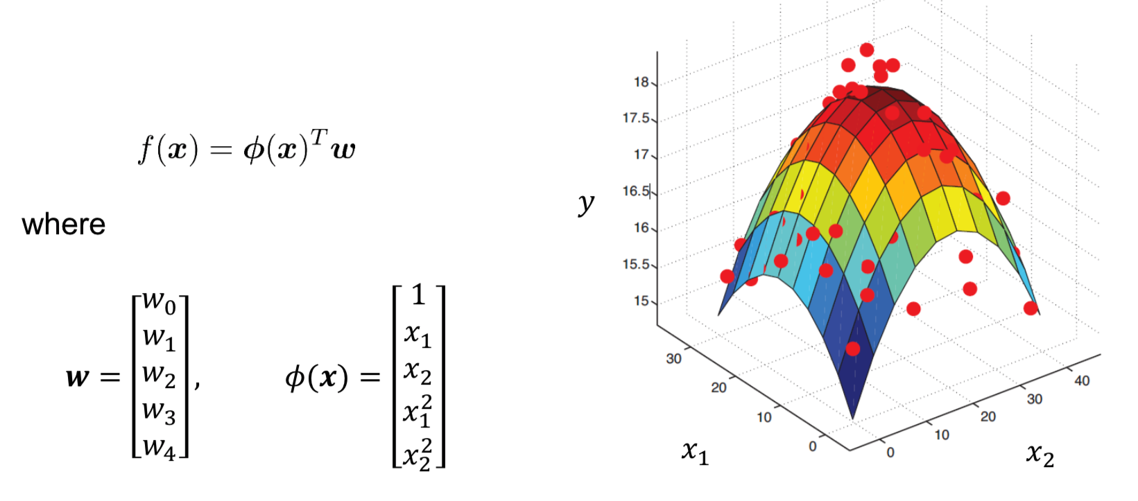
Example 2

$\boldsymbol{x}=\left[\begin{array}{c}{x_1 \\ x_2}\end{array}\right] \in \mathbb{R}^{2}$

$\phi: \mathbb{R}^2 \to \mathbb{R}^5, \left[\begin{array}{c}{x_1 \\ x_2}\end{array}\right] \mapsto \left[\begin{array}{c}{1 \\ x_1 \\ x_2 \\ x_1^2 \\ x_2^2}\end{array}\right]$

Optimal value of $\boldsymbol{w}$

$\boldsymbol{w}^{*}=\left(\boldsymbol{\Phi}^{T} \boldsymbol{\Phi}\right)^{-1} \boldsymbol{\Phi}^{T} \boldsymbol{y}, \qquad \mathbf{\Phi}=\left[\begin{array}{c}{\phi_{1}^{T}} \\\\ {\vdots} \\\\ {\phi_{n}^{T}}\end{array}\right]$

(The same as in Linear Regression, just the data matrix is now replaced by the basis function matrix)

Challenge of Polynomial Regression: Overfitting

Reason: Too complex model (Degree of the polynom is too high!). It fits the noise and has unspecified behaviour between the training points.😭

Solution: Regularization

Regularization

Regularization: Constrain a model to make it simpler and reduce the task of overfitting.

💡 Avoid overfitting by forcing the weights $\boldsymbol{w}$ to be small

Assume that our model has degree of 3 ($x^1, x^2, x^3$), and the corresponding parameters/weights are $w_1, w_2, w_3$. If we force $w_3=0$, then $w_3 x^3 = 0$, meaning that the model now has only degree of 2. In other words. the model is somehow simpler.

In general, a regularized model has the following cost/objective function:

$\lambda$: regularization factor (hyperparameter, need to be tuned manually), controls how much you want to regularize the model.

Regularized Least Squares (Ridge Regression)

Consists of:

• Sum of Squareds Error (SSE) function
• quadratic regulariser ($L_2$-Regularization)

$\begin{aligned} L_{\text {ridge }} &= \mathbf{SSE} + \lambda \|w\|^2 \\\\ &= (\boldsymbol{y}-\boldsymbol{\Phi} \boldsymbol{w})^{T}(\boldsymbol{y}-\boldsymbol{\Phi} \boldsymbol{w})+\lambda \boldsymbol{w}^{T} \boldsymbol{w} \end{aligned}$

Solution:

$\boldsymbol{w}_{\mathrm{ridge}}^{*}=\left(\boldsymbol{\Phi}^{T} \boldsymbol{\Phi}+\lambda \boldsymbol{I}\right)^{-1} \boldsymbol{\Phi}^{T} \boldsymbol{y}$

• $\boldsymbol{I}$: Identity matrix
• $\left(\boldsymbol{\Phi}^{T} \boldsymbol{\Phi}+\lambda \boldsymbol{I}\right)$ is full rank and can be easily inverted