Gaussian Mixture Model
Gaussian Distribution
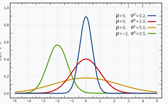
Univariate: The Probability Density Function (PDF) is:
$$ P(x | \theta)=\frac{1}{\sqrt{2 \pi \sigma^{2}}} \exp \left(-\frac{(x-\mu)^{2}}{2 \sigma^{2}}\right) $$- $\mu$: mean
- $\sigma$: standard deviation
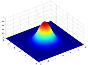
Multivariate: The Probability Density Function (PDF) is:
$$ P(x | \theta)=\frac{1}{(2 \pi)^{\frac{D}{2}}|\Sigma|^{\frac{1}{2}}} \exp \left(-\frac{(x-\mu)^{T} \Sigma^{-1}(x-\mu)}{2}\right) $$- $\mu$: mean
- $\Sigma$: covariance
- $D$: dimension of data
Learning
For univariate Gaussian model, we can use Maximum Likelihood Estimation (MLE) to estimate parameter $\theta$ :
$$ \theta= \underset{\theta}{\operatorname{argmax}} L(\theta) $$Assuming data are i.i.d, we have:
$$ L(\theta)=\prod\_{j=1}^{N} P\left(x\_{j} | \theta\right) $$For numerical stability, we usually use Maximum Log-Likelihood:
$$ \begin{align} \theta &= \underset{\theta}{\operatorname{argmax}} L(\theta) \\\\ &= \underset{\theta}{\operatorname{argmax}} \log(L(\theta)) \\\\ &= \underset{\theta}{\operatorname{argmax}} \sum\_{j=1}^{N} \log P\left(x\_{j} | \theta\right)\end{align} $$Gaussian Mixture Model
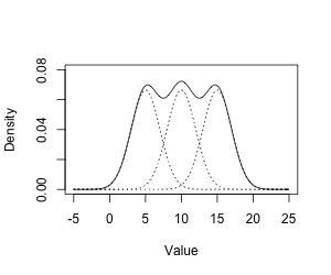
A Gaussian mixture model is a probabilistic model that assumes all the data points are generated from a mixture of a finite number of Gaussian distributions with unknown parameters. One can think of mixture models as generalizing k-means clustering to incorporate information about the covariance structure of the data as well as the centers of the latent Gaussians.
Define:
$x\_j$: the $j$-th observed data, $j=1, 2,\dots, N$
$K$: number of Gaussian model components
$\alpha\_k$: probability that the observed data belongs to the $k$-th model component
- $\alpha\_k \geq 0$
- $\displaystyle \sum\_{k=1}^{K}\alpha\_k=1$
$\phi(x|\theta\_k)$: probability density function of the $k$-th model component
- $\theta\_k = (\mu\_k, \sigma\_k^2)$
$\gamma\_{jk}$: probability that the $j$-th obeserved data belongs to the $k$-th model component
Probability density function of Gaussian mixture model:
$$ P(x | \theta)=\sum\_{k=1}^{K} \alpha\_{k} \phi\left(x | \theta\_{k}\right) $$For this model, parameter is $\theta=\left(\tilde{\mu}\_{k}, \tilde{\sigma}\_{k}, \tilde{\alpha}\_{k}\right)$.
Expectation-Maximum (EM)
Expectation-Maximization (EM) is a statistical algorithm for finding the right model parameters. We typically use EM when the data has missing values, or in other words, when the data is incomplete.
These missing variables are called latent variables.
- NEVER observed
- We do NOT know the correct values in advance
Since we do not have the values for the latent variables, Expectation-Maximization tries to use the existing data to determine the optimum values for these variables and then finds the model parameters. Based on these model parameters, we go back and update the values for the latent variable, and so on.
The Expectation-Maximization algorithm has two steps:
- E-step: In this step, the available data is used to estimate (guess) the values of the missing variables
- M-step: Based on the estimated values generated in the E-step, the complete data is used to update the parameters
EM in Gaussian Mixture Model
Initialize the parameters ($K$ Gaussian distributionw with the mean $\mu\_1, \mu\_2,\dots,\mu\_k$ and covariance $\Sigma\_1, \Sigma\_2, \dots, \Sigma\_k$)
Repeat
- E-step: For each point $x\_j$, calculate the probability that it belongs to cluster/distribution $k$
The value will be high when the point is assigned to the right cluster and lower otherwise
- M-step: update parameters
until convergence ($\left\|\theta\_{i+1}-\theta\_{i}\right\|<\varepsilon$)
Visualization:
