Principle Components Analysis (PCA)

TL;DR

The usual procedure to calculate the $d$-dimensional principal component analysis consists of the following steps:

0. Calculate

   • average

     $$ \bar{m}=\sum\_{i=1}^{N} m_{i} \in \mathbb{R} $$

   • data matrix

     $$ \mathbf{M}=\left(m\_{1}-\bar{m}, \ldots, m\_{N}-\bar{m}\right) \in \mathbb{R}^{d \times \mathrm{N}} $$

   • scatter matrix (covariance matrix)

     $$ \mathbf{S}=\mathbf{M M}^{\mathrm{T}} \in \mathbb{R}^{d \times d} $$

   of all feature vectors $m\_{1}, \ldots, m\_{N}$

1. Calculate the normalized ($\\|\cdot\\|=1$) eigenvectors $\mathbf{e}\_1, \dots, \mathbf{e}\_d$ and sort them such that the corresponding eigenvalues $\lambda\_1, \dots, \lambda\_d$ are decreasing, i.e. $\lambda\_1 > \lambda\_2 > \dots > \lambda\_d$

2. Construct a matrix

   $$ \mathbf{A}:=\left(e\_{1}, \ldots, e\_{d^{\prime}}\right) \in \mathbb{R}^{d \times d^{\prime}} $$

   with the first $d^{\prime}$ eigenvectors as its columns

3. Transform each feature vector $m\_i$ into a new feature vector

   $$ \mathrm{m}\_{\mathrm{i}}^{\prime}=\mathrm{A}^{\mathrm{T}}\left(\mathrm{m}\_{\mathrm{i}}-\overline{\mathrm{m}}\right) \quad \text { for } i=1, \ldots, N $$

   of smaller dimension $d^{\prime}$

Dimensionality reduction

• Goal: represent instances with fewer variables

  • Try to preserve as much structure in the data as possible
  • Discriminative: only structure that affects class separability

• Feature selection

  • Pick a subset of the original dimensions
  • Discriminative: pick good class “predictors”

• Feature extraction

  • Construct a new set of dimensions

    $$ E\_{i} = f(X\_1 \dots X\_d) $$
    • $X\_1, \dots, X\_d$: features

  • (Linear) combinations of original

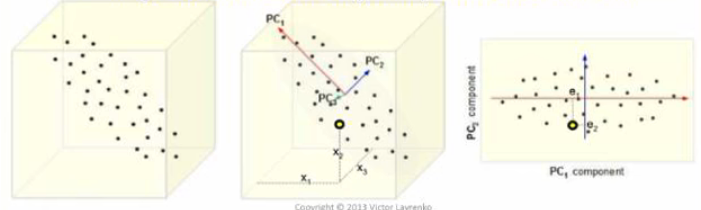
Direction of greatest variance

• Define a set of principal components
  • 1st: direction of the greatest variability in the data (i.e. Data points are spread out as far as possible)
  • 2nd: perpendicular to 1st, greatest variability of what’s left
  • …and so on until $d$ (original dimensionality)
• First $m \ll d$ components become $m$ dimensions
  • Change coordinates of every data point to these dimensions

How to PCA?

1. “Center” the data at zero (subtract mean from each attribute)

   $$ x\_{i, a} = x\_{i, a} - \mu $$

2. Compute covariance matrix $\Sigma$

   The covariance between two attributes is an indication of whether they change together (positive correlation) or in opposite directions (negative correlation).

   For example, $cov(x\_1, x\_2) = 0.8 > 0 \Rightarrow$ When $x\_1$ increases/decreases, $x\_2$ also increases/decreases.

   $$ cov(b, a) = \frac{1}{n} \sum\_{i=1}^{n} x\_{ib} x\_{ia} $$

3. We want vectors $\mathbf{e}$ which aren’t turned by covariance matrix $\Sigma$:

   $$ \Sigma \mathbf{e} = \lambda \mathbf{e} $$

   $\Rightarrow$ $\mathbf{e}$ are eigenvectors of $\Sigma$, and $\lambda$ are corresponding eigenvalues

   Principle components = eigenvectors with largest eigenvalues

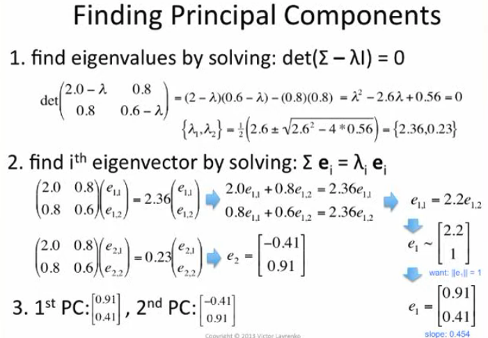
Finding principle components

1. Find eigenvalues by solving Characteristic Polynomial

   $$ \operatorname{det}(\Sigma - \lambda \mathbf{I}) = 0 $$
   • $\mathbf{I}$: Identity matrix

2. Find $i$-th eigenvector by solving

   $$ \Sigma \mathbf{e}\_i = \lambda\_i \mathbf{e}\_i $$

   and we want $\mathbf{e}\_{i}$ to have unit length ($\\|\mathbf{e}\_{i}\\| = 1$)

3. Eigenvector with the largest eigenvalue will be the first principle component, eigenvector with the second largest eigenvalue will be the second priciple component, so on and so on.

Example

Projecting to new dimension

• We pick $m

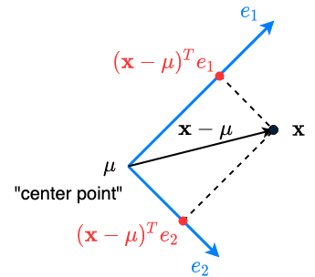
• For instance $\mathbf{x} = \{x\_1, \dots, x\_d\}$ (original coordinates), we want new coordinates $\mathbf{x}^{\prime} = \{x^{\prime}\_1, \dots, x^{\prime}\_d\}$

  • “Center” the instance (subtract the mean): $\mathbf{x} - \mathbf{\mu}$
  • “Project” to each dimension: $(\mathbf{x} - \mathbf{\mu})^T \mathbf{e}\_j$ for $j=1, \dots, m$
  Example

  

Go deeper in details

Why eigenvectors = greatest variance?

Why eigenvalue = variance along eigenvector?

How many dimensions should we reduce to?

• Now we have eigenvectors $\mathbf{e}\_1, \dots, \mathbf{e}\_d$ and we want new dimension $m \ll d$

• We pick $\mathbf{e}\_i$ that “explain” the most variance:

  • Sort eigenvectors s.t. $\lambda\_1 \geq \dots \geq \lambda\_d$

  • Pick first $m$ eigenvectors which explain 90% or the total variance (typical threshold values: 0.9 or 0.95)

    

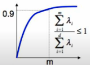
• Or we can use a scree plot

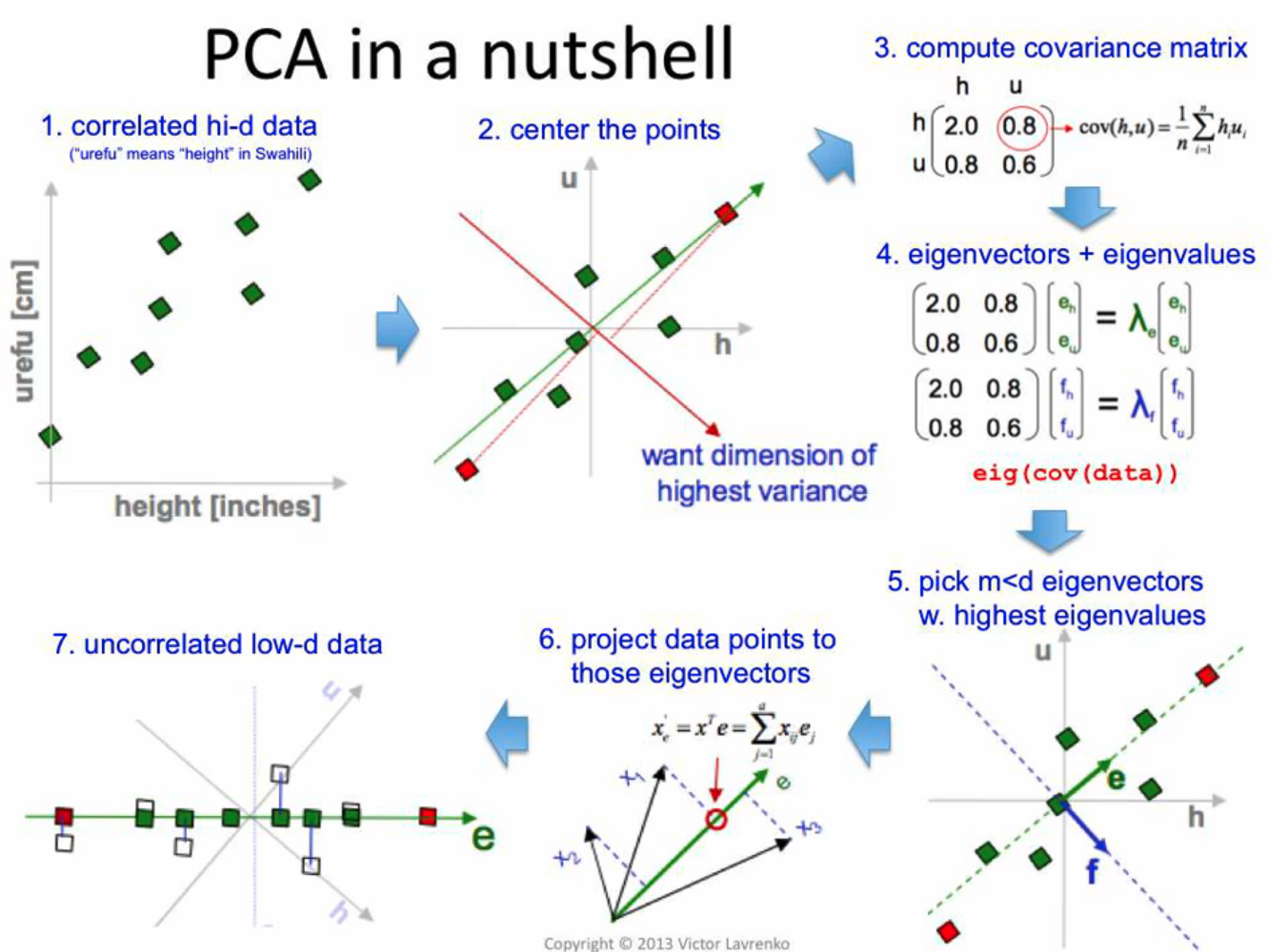
PCA in a nutshell

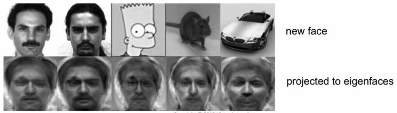
PCA example: Eigenfaces

Perform PCA on bitmap images of human faces:

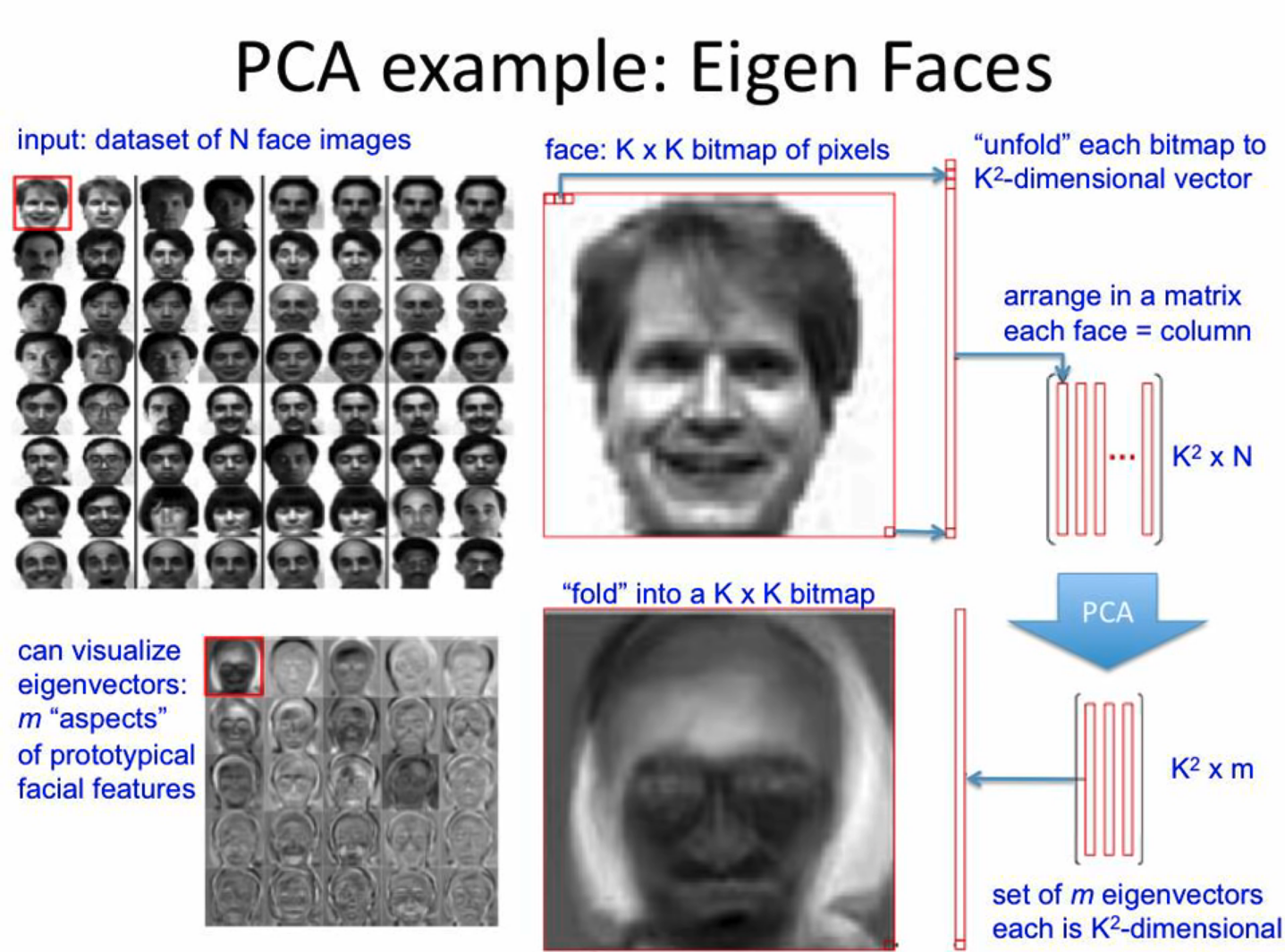
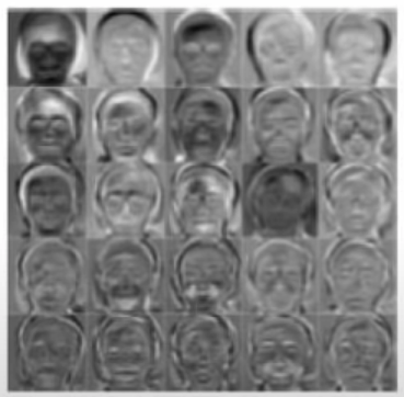
Belows are the eigenvectors after we perform PCA on the dataset:

Then we can project new face to space of eigen-faces, and represent vector of new face as a linear combination of principle components.

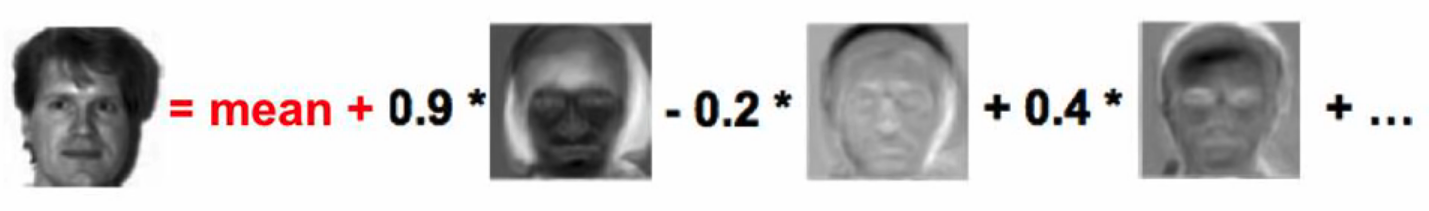
As we use more and more eigenvectors in this decomposition, we can end up with a face that looks more and more like the original guy

Application of eigenface

• Face similarity

  • in the reduced space
  • insensitive to lighting expression, orientation

• Projecting new “faces”

  

Pratical issues of PCA

• PCA is based on covariance matrix and covariance is extremely sensitive to large values

  • E.g. multiple some dimension by 1000. Then this dimension dominates covariance and become a principle component.

  • Solution: normalize each dimension to zero mean and unit variacne

    $$ x^{\prime} = \frac{x - \text{mean}}{\text{standard deviation}} $$

• PCA assumes underlying subspace is linear.

• PCA can sometimes hurt the performace of classification

  • Because PCA doesn’t see the labels

  • Solution: Linear Discriminant Analysis (LDA)

    • Picks a new dimension that gives

      • maximum separation between means of prejected classes
      • minimum variance within each projected class

      

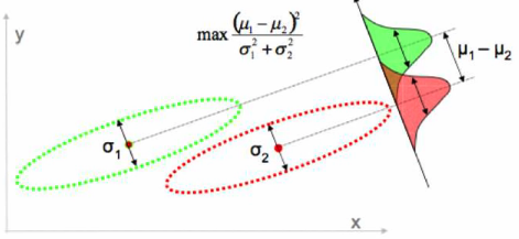
    • But this relies on some assumptions of the data and does not always work. 🤪

Reference

• Principle Component Analysis: a great series of video tutorials explaining PCA clearly 👍