04-NER

Named Entity Recognition

Introduction

Definition

Named Entity: some entity represented by a name

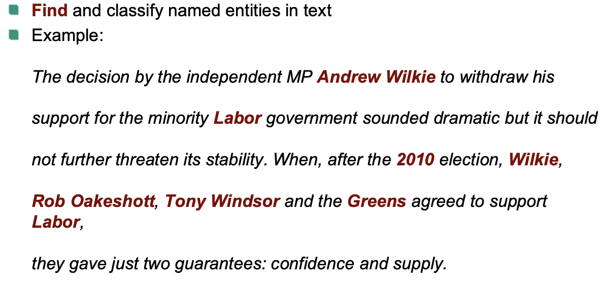
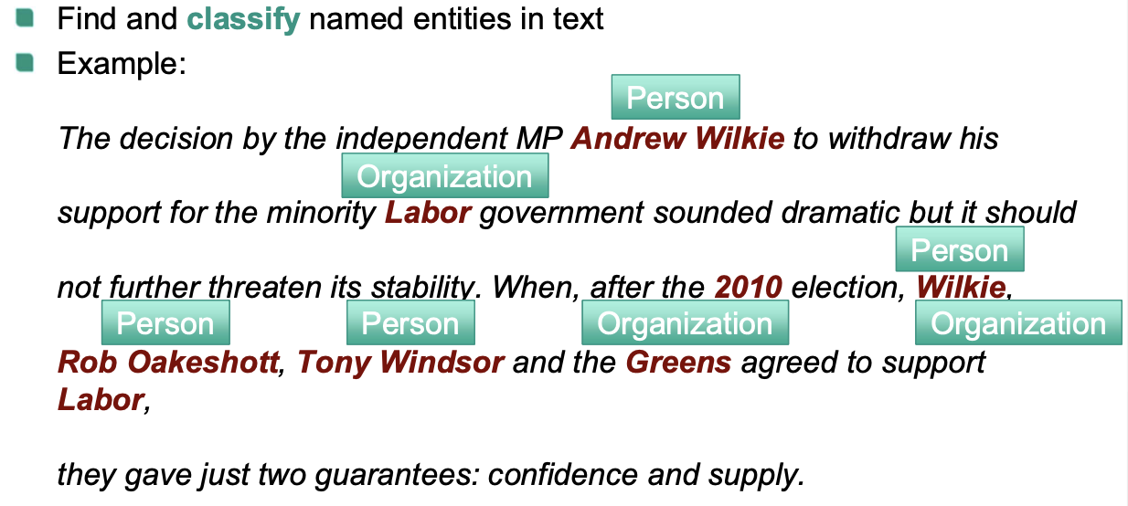
Named Entity Recognition: Find and classify named entities in text

Why useful?

Create indices & hyperlinks
Information extraction
- Establish relationships between named entities, build knowledge base
Question answering: answers often NEs
Machine translation: NEs require special care
- NEs often unknown words, usually passed through without translation.

Why difficult?

World knowledge
Non-local decisions
Domain specificity
Labeled data is very expensive

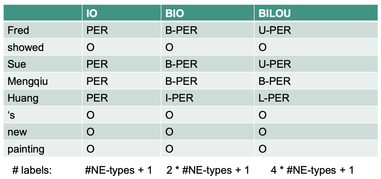
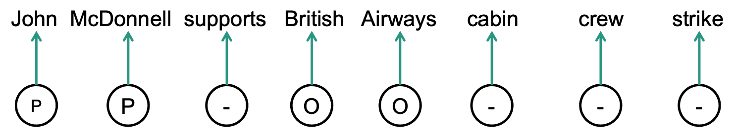
Label Representation

IO
- I: Inside
- O: Outside (indicates that a token belongs to no chunk)
BIO
- B: Begin
  Wiki
  The IOB format (short for inside, outside, beginning), a synonym for BIO format, is a common tagging format for tagging tokens in a chunking task in computational linguistics.
  - B-prefix before a tag: indicates that the tag is the beginning of a chunk
  - I-prefix before a tag: indicates that the tag is the inside of a chunk
  - O tag: indicates that a token belongs to NO chunk
BIOES
- E: Ending character
- S: single element
BILOU
- L: Last character
- U: Unit length

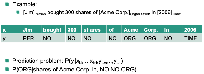
Example:

Fred showed Sue Mengqiu Huang's new painting

Data

CoNLL03 shared task data
MUC7 dataset
Guideline examples for special cases:
- Tokenization
- Elision

Evaluation

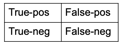
Precision and Recall
$\text{Precision} = \frac{\\# \text { correct labels }}{\\# \text { hypothesized labels }} = \frac{TP}{TP + FP}$ $\text{Recall} = \frac{\\# \text { correct labels }}{\\# \text { reference labels }} = \frac{TP}{TP + FN}$
- Phrase-level counting
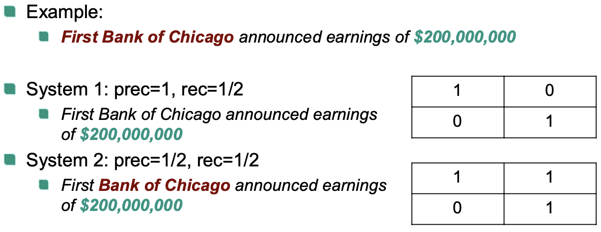
  - System 1:
    - “ $\text{\\$200,000,000}$ " is correctly recognized as NE $\Rightarrow$ TP =1
    - “First Bank of Chicago” is incorrectly recognised as non-NE (i.e., O) $\Rightarrow$ FN = 1
    Therefore:
    - $\text{Precision} = \frac{1}{1 + 0} = 1$
      $\text{Recall} = \frac{1}{1 + 1} = \frac{1}{2}$
  - System 2:
    - “ $\text{\\$200,000,000}$ " is correctly recognized as NE $\Rightarrow$ TP =1
    - For “First Bank of Chicago”
      Word Actual label Predicted label
      First ORG O
      Bank of Chicago ORG ORG
      There’s a boundary error (since we consider the whole phrase):
      FN = 1
      FP = 1
    Therefore:
    - $\text{Precision} = \frac{1}{1 + 1} = \frac{1}{2}$
    - $\text{Recall} = \frac{1}{1 + 1} = \frac{1}{2}$
  - Problems
    - Punish partial overlaps
    - Ignore true negatives
- Token-level
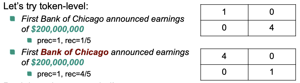
  In token-level, we consider these tokens: “First”, “Bank”, “of”, “Chicago”, and “$200,000,000”
  - System 1
    - “ $\text{\\$200,000,000}$ " is correctly recognized as NE $\Rightarrow$ TP =1
    - “First”, “Bank”, “of”, “Chicago” are incorrectly recognised as non-NE (i.e., O) $\Rightarrow$ FN = 4
    Therefore:
    - $\text{Precision} = \frac{1}{1 + 0} = 1$
    - $\text{Recall} = \frac{1}{1 + 4} = \frac{1}{5}$
  - Partial overlaps rewarded!
  - But
    - longer entities weighted more strongly
    - True negatives still ignored 🤪
$F\_1$ score (harmonic mean of precision and recall)
$F\_1 = \frac{2 \times \text { precision } \times \text { recall }}{\text { precision }+\text { recall }}$

Word	Actual label	Predicted label
First	ORG	O
Bank of Chicago	ORG	ORG

Text Representation

Local features

Previous two predictions (tri-gram feature)
- $y\_{i-1}$ and $y\_{i-2}$
Current word $x\_i$
Word type $x\_i$
- all-capitalized, is-capitalized, all-digits, alphanumeric, …
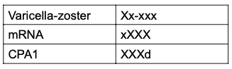
Word shape
- lower case - ‘x’
- upper case - ‘X’
- numbers - ’d'
- retain punctuation
Word substrings
Tokens in window
Word shapes in window
…

Non-local features

Identify tokens that should have same labels

Type:

Context aggregation
- Derived from all words in the document
- No dependencies on predictions, usable with any inference algorithm
Prediction aggregation
- Derived from predictions of the whole document
- Global dependencies; Inference:
  - first apply baseline without non-local features
  - then apply second system conditioned on output of first system
Extended prediction history
- Condition only on past predictions –> greedy / beam search
- 💡 Intuition: Beginning of document often easier, later in document terms often get abbreviated

Sequence Model

HMMs

Generative model
Generative story:
- Choose document length $N$
- For each word $t = 0, \dots, N$ :
  - Draw NE label $\sim P(y\_t | y\_{t-1})$
  - Draw word $\sim P\left(x\_{t} | y\_{t}\right)$
    $P(\mathbf{y}, \mathbf{x})=\prod P\left(y\_{t} | y\_{t-1}\right) P\left(x | y\_{t}\right)$
Example
👍 Pros
- intuitive model
- Works with unknown label sequences
- Fast inference
👎 Cons
- Strong limitation on textual features (conditional independence)
- Model overly simplistic (can improve the generative story but would lose fast inference)

Max. Entropy

Discriminative model $P(y\_t|x)$
Don’t care about generation process or input distribution
Only model conditional output probabilities
👍 Pros: Flexible feature design
👎 Cons: local classifier -> disregard sequence information

CRF

Discriminative model
👍 Pros:
- Flexible feature design
- Condition on local sequence context
- Training as easy as MaxEnt
👎 Cons: Still no long-range dependencies possible

Modelling

Difference to POS

Long-range dependencies
Alternative resources can be very helpful
Several NER more than one word long

Example

Inference

Viterbi

Finds exact solution
Efficient algorithmic solution using dynamic programming
Complexity exponential in order of Markov model
- Only feasible for small order

Greedy

At each timestep, choose locally best label
Fast, support conditioning on global history (not future)
No possibility for “label revision”

Beam

Keep a beam of the $n$ best greedy solutions, expand and prune
Limited room for label revisions

Gibbs Sampling

Stochastic method
Easy way to sample from multivariate distribution
Normally used to approximate joint distributions or intervals
$P\left(y^{(t)} | y^{(t-1)}\right)=P\left(y\_{i}^{(t)} | y\_{-i}^{(t-1)}, x\right)$
- $-1$ means all states except $i$
💡 Intuitively:
- Sample one variable at a time, conditioned on current assignment of all other variables
- Keep checkpoints (e.g. after each sweep through all variables) to approximate distribution
In our case:
- Initialize NER tags (e.g. random or via Viterbi baseline model)
- Re-sample one tag at a time, conditioned on input and all other tags
- After sampling for a long time, we can estimate the joint distribution over outputs $P(y|x)$
- However, it’s slow, and we may only be interested in the best output 🤪
- Could choose best instead of sampling
  $y^{(t)}=y\_{-i}^{(t-1)} \cup \underset{y\_{i}^{(t)}}{\operatorname{argmax}}\left(P\left(y\_{i}^{(t)} | y\_{-i}^{(t-1)}, x\right)\right)$
  - will get stuck in local optima 😭
- Better: Simulated annealing
  - Gradually move from sampling to argmax $P\left(y^{(t)} | y^{(t-1)}\right)=\frac{P\left(y\_{i}^{(t)} | y\_{-i}^{(t-1)}, x\right)^{1 / c\_{t}}}{\displaystyle\sum\_{j} P\left(y\_{j}^{(t)} | y\_{-j}^{(t-1)}, x\right)^{1 / c\_{t}}}$

External Knowledge

Data

Supervised learning:
- Label Data:
  - Text
  - NE Annotation
Unsupervised learning
- Unlabeled Data: Text
- Problem: Hard to directly learn NER
Semi-supervised: Labeled and Unlabeled Data

Word Clustering

Problem: Data Sparsity
Idea
- Find lower-dimensional representation of words
- real vector /probabilities have natural measure of similarity
Which words are similarr?
- Distributional notion
- if they appear in similar context, e.g.
  - “president” and “chairman” are similar
  - “cut” and “knife” not

Words in same cluster should be similar

Brown clusters

Bottom-up agglomerative word clustering
Input: Sequence of words $w\_1, \dots, w\_n$
Output
- binary tree
- Cluster: subtree (according to desired #clusters)
💡 Intuition: put syntacticly “exchangable” words in same cluster. E.g.:
- Similar words: president/chairman, Saturday/Monday
- Not similar: cut/knife
Algorithm:
- Initialization: Every word is its own cluster
- While there are more than one cluster
  - Merge two clusters that maximizes the quality of the clustering
Result:
- Hard clustering: each word belongs to exactly one cluster
Quality of the clustering
- Use class-based bigram language model
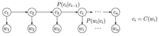
- Quality: logarithm of the probability of the training text normalized by the length of the text
  $\begin{aligned} \text { Quality }(C) &=\frac{1}{n} \log P\left(w\_{1}, \ldots, w\_{n}\right) \\\\ &=\frac{1}{n} \log P\left(w\_{1}, \ldots, w\_{n}, C\left(w\_{1}\right), \ldots, C\left(w\_{n}\right)\right) \\\\ &=\frac{1}{n} \log \prod\_{i=1}^{n} P\left(C\left(w\_{i}\right) | C\left(w\_{i-1}\right)\right) P\left(w\_{i} | C\left(w\_{i}\right)\right) \end{aligned}$
- Parameters: estimated using maximum-likelihood

Last updated on 2024-09-05

← Part-of-Speech Tagging 2020-09-15

Parsing 2020-09-15 →