Gradient Descent

Overview

🎯 Goal with gradient descent: find the optimal weights that minimize the loss function we’ve defined for the model.

From now on, we’ll explicitly represent the fact that the loss function $L$ is parameterized by the weights $\theta$ (in the case of logistic regression $\theta=(w, b)$):

$$ \hat{\theta}=\underset{\theta}{\operatorname{argmin}} \frac{1}{m} \sum\_{i=1}^{m} L_{C E}\left(y^{(i)}, x^{(i)} ; \theta\right) $$

Gradient descent finds a minimum of a function by figuring out in which direction (in the space of the parameters $\theta$) the function’s slope is rising the most steeply, and moving in the opposite direction.

💡 Intuition

if you are hiking in a canyon and trying to descend most quickly down to the river at the bottom, you might look around yourself 360 degrees, find the direction where the ground is sloping the steepest, and walk downhill in that direction.

For logistic regression, this loss function is conveniently convex

• Just one minimum
• No local minima to get stuck in

$\Rightarrow$ Gradient descent starting from any point is guaranteed to find the minimum. 👏

Visualization:

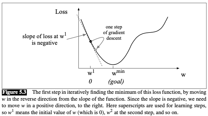
The magnitude of the amount to move in gradient descent is the value of the slope $\frac{d}{d w} f(x ; w)$ weighted by a learning rate $\eta$. A higher (faster) learning rate means that we should move w more on each step.

In the single-variable example above, The change we make in our parameter is

$$ w^{t+1}=w^{t}-\eta \frac{d}{d w} f(x ; w) $$

In $N$-dimensional space, the gradient is a vector that expresses the directinal components of the sharpest slope along each of those $N$ dimensions.

Visualizaion (E.g., $N=2$):

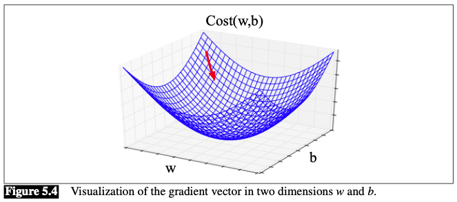
In each dimension $w_i$, we express the slope as a partial derivative $\frac{\partial}{\partial w_i}$ of the loss function. The gradient is defined as a vector of these partials:

$$ \left.\nabla_{\theta} L(f(x ; \theta), y)\right)=\left[\begin{array}{c} \frac{\partial}{\partial w_{1}} L(f(x ; \theta), y) \\\\ \frac{\partial}{\partial w_{2}} L(f(x ; \theta), y) \\\\ \vdots \\\\ \frac{\partial}{\partial w_{n}} L(f(x ; \theta), y) \end{array}\right] $$

Thus, the change of $\theta$ is:

$$ \theta_{t+1}=\theta_{t}-\eta \nabla L(f(x ; \theta), y) $$

The gradient for Logistic Regression

For logistic regression, the cross-entropy loss function is

$$ L_{C E}(w, b)=-[y \log \sigma(w \cdot x+b)+(1-y) \log (1-\sigma(w \cdot x+b))] $$

The derivative of this loss function is:

$$ \frac{\partial L_{C E}(w, b)}{\partial w_{j}}=[\sigma(w \cdot x+b)-y] x_{j} $$

For derivation of the derivative above we need:

• derivative of $\ln(x)$:

  $$ > \frac{d}{d x} \ln (x)=\frac{1}{x} > $$

• derivative of the sigmoid:

  $$ > \frac{d \sigma(z)}{d z}=\sigma(z)(1-\sigma(z)) > $$

• Chain rule of derivative: for $f(x)=u(v(x))$,

  $$ > \frac{d f}{d x}=\frac{d u}{d v} \cdot \frac{d v}{d x} > $$

Now compute the derivative:

$$ > \begin{aligned} > \frac{\partial L L(w, b)}{\partial w_{j}} &=\frac{\partial}{\partial w_{j}}-[y \log \sigma(w \cdot x+b)+(1-y) \log (1-\sigma(w \cdot x+b))] \\\\ > &=-\frac{\partial}{\partial w_{j}} y \log \sigma(w \cdot x+b) - \frac{\partial}{\partial w_{j}}(1-y) \log [1-\sigma(w \cdot x+b)] \\\\ > &\overset{\text{chain rule}}{=} -\frac{y}{\sigma(w \cdot x+b)} \frac{\partial}{\partial w_{j}} \sigma(w \cdot x+b)-\frac{1-y}{1-\sigma(w \cdot x+b)} \frac{\partial}{\partial w_{j}} 1-\sigma(w \cdot x+b)\\\\ > &= -\left[\frac{y}{\sigma(w \cdot x+b)}-\frac{1-y}{1-\sigma(w \cdot x+b)}\right] \frac{\partial}{\partial w_{j}} \sigma(w \cdot x+b) \\\\ > \end{aligned} > $$

Now plug in the derivative of the sigmoid, and use the chain rule one more time:

$$ > \begin{aligned} > \frac{\partial L L(w, b)}{\partial w_{j}} &=-\left[\frac{y-\sigma(w \cdot x+b)}{\sigma(w \cdot x+b)[1-\sigma(w \cdot x+b)]}\right] \sigma(w \cdot x+b)[1-\sigma(w \cdot x+b)] \frac{\partial(w \cdot x+b)}{\partial w_{j}} \\\\ > &=-\left[\frac{y-\sigma(w \cdot x+b)}{\sigma(w \cdot x+b)[1-\sigma(w \cdot x+b)]}\right] \sigma(w \cdot x+b)[1-\sigma(w \cdot x+b)] x_{j} \\\\ > &=-[y-\sigma(w \cdot x+b)] x_{j} \\\\ > &=[\sigma(w \cdot x+b)-y] x_{j} > \end{aligned} > $$

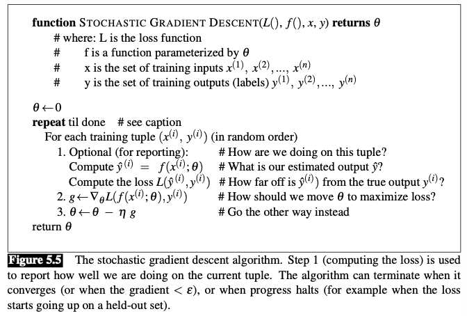
Stochastic Gradient descent

Stochastic gradient descent is an online algorithm that minimizes the loss function by

• computing its gradient after each training example, and
• nudging $\theta$ in the right direction (the opposite direction of the gradient).

The learning rate η is a (hyper-)parameter that must be adjusted.

• If it’s too high, the learner will take steps that are too large, overshooting the minimum of the loss function.
• If it’s too low, the learner will take steps that are too small, and take too long to get to the minimum.

It is common to begin the learning rate at a higher value, and then slowly decrease it, so that it is a function of the iteration $k$ of training.

Mini-batch training

Stochastic gradient descent: chooses a single random example at a time, moving the weights so as to improve performance on that single example.

• Can result in very choppy movements

Batch gradient descent: compute the gradient over the entire dataset.

• Offers a superb estimate of which direction to move the weights
• Spends a lot of time processing every single example in the training set to compute this perfect direction.

Mini-batch gradient descent

• we train on a group of $m$ examples (perhaps 512, or 1024) that is less than the whole dataset.
• Has the advantage of computational efficiency
  • The mini-batches can easily be vectorized, choosing the size of the mini-batch based on the computational resources.
  • This allows us to process all the exam- ples in one mini-batch in parallel and then accumulate the loss

Define the mini-batch version of the cross-entropy loss function (assuming the training examples are independent):

$$ \begin{aligned} \log p(\text {training labels}) &=\log \prod\_{i=1} p\left(y^{(i)} | x^{(i)}\right) \\\\ &=\sum\_{i=1}^{m} \log p\left(y^{(i)} | x^{(i)}\right) \\\\ &=-\sum\_{i=1}^{m} L\_{C E}\left(\hat{y}^{(i)}, y^{(i)}\right) \end{aligned} $$

The cost function for the mini-batch of $m$ examples is the average loss for each example:

$$ \begin{aligned} \operatorname{cost}(w, b) &=\frac{1}{m} \sum\_{i=1}^{m} L_{C E}\left(\hat{y}^{(i)}, y^{(i)}\right) \\\\ &=-\frac{1}{m} \sum\_{i=1}^{m} y^{(i)} \log \sigma\left(w \cdot x^{(i)}+b\right)+\left(1-y^{(i)}\right) \log \left(1-\sigma\left(w \cdot x^{(i)}+b\right)\right) \end{aligned} $$

The mini-batch gradient is the average of the individual gradients:

$$ \frac{\partial \operatorname{cost}(w, b)}{\partial w_{j}}=\frac{1}{m} \sum_{i=1}^{m}\left[\sigma\left(w \cdot x^{(i)}+b\right)-y^{(i)}\right] x_{j}^{(i)} $$