Sigmoid

Sigmoid to Logistic Regression

Consider a single input observation $x = [x_1, x_2, \dots, x_n]$

The classifier output $y$ can be

• $1$: the observation is a member of the class
• $0$: the observation is NOT a member of the class

We want to know the probability $P(y=1|x)$ that this observation is a member of the class.

E.g.:

• The decision is “positive sentiment” versus “negative sentiment”
• the features represent counts of words in a document
• $P(y=1|x)$ is the probability that the document has positive sentiment, while and $P(y=0|x)$ is the probability that the document has negative sentiment.

Logistic regression solves this task by learning, from a training set, a vector of weights and a bias term.

• Each weight $w_i$ is a real number, and is associated with one of the input features $x_i$. The weight represents how important that input feature is to the classification decision, can be

  • positive (meaning the feature is associated with the class)
  • negative (meaning the feature is NOT associated with the class).

  E.g.: we might expect in a sentiment task the word awesome to have a high positive weight, and abysmal to have a very negative weight.

• Bias term $b$, also called the intercept, is another real number that’s added to the weighted inputs.

To make a decision on a test instance, the resulting single number $z$ expresses the weighted sum of the evidence for the class:

(Note that $z$ is NOT a legal probability, since $z \notin [0, 1]$)

To create a probability, we’ll pass $z$ through the sigmoid function (also called logistic function):

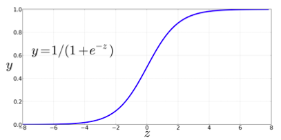
👍 Advantages of sigmoid

• It takes a real-valued number and maps it into the range [0,1] (which is just what we want for a probability)
• It is nearly linear around 0 but has a sharp slope toward the ends, it tends to squash outlier values toward 0 or 1.
• Differentiable $\Rightarrow$ handy for learning

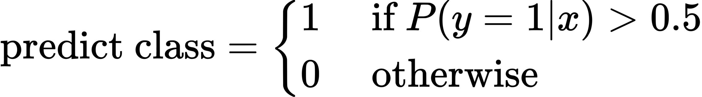
To make it a probability, we just need to make sure that the two cases, $P(y=1)$ and $P(y=0)$, sum to 1:

Now we have an algorithm that given an instance $x$ computes the probability $P(y=1|x)$. For a test instance $x$, we say yes if the probability is $P(y=1|x)$ more than 0.5, and no otherwise. We call 0.5 the decision boundary:

Example: sentiment classification

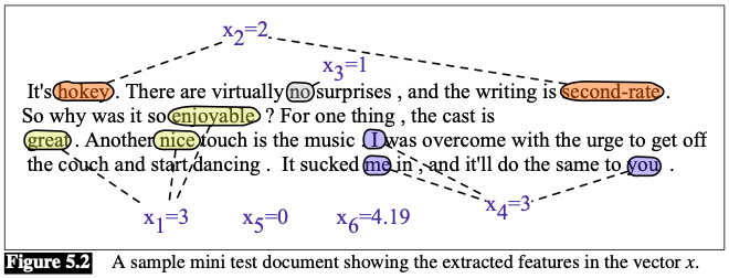
Suppose we are doing binary sentiment classification on movie review text, and we would like to know whether to assign the sentiment class + or − to a review document $doc$.

We’ll represent each input observation by the 6 features $x_1,...,x_6$ of the input shown in the following table

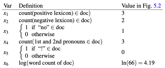
Assume that for the moment that we’ve already learned a real-valued weight for each of these features, and that the 6 weights corresponding to the 6 features are $w= [2.5,−5.0,−1.2,0.5,2.0,0.7]$, while $b = 0.1$.

• The weight $w_1$, for example indicates how important a feature the number of positive lexicon words (great, nice, enjoyable, etc.) is to a positive sentiment decision, while $w_2$tells us the importance of negative lexicon words. Note that $w_1 = 2.5$ is positive, while $w_2 = −5.0$, meaning that negative words are negatively associated with a positive sentiment decision, and are about twice as important as positive words.

Given these 6 features and the input review $x$, $P(+|x)$ and $P(-|x)$ can be computed:

$0.70 > 0.50 \Rightarrow$ This sentiment is positive ($+$).