Train Naive Bayes Classifiers

Maximum Likelihood Estimate (MLE)

In Naive Bayes calculation we have to learn the probabilities $P(c)$ and $P(w_i|c)$. We use the Maximum Likelihood Estimate (MLE) to estimate them. We’ll simply use the frequencies in the data.

• $P(c)$: document prior

  • “what percentage of the documents in our training set are in each class $c$ ?”
  $$\hat{P}(c)=\frac{N_{c}}{N_{d o c}}$$
  • $N_c$: the number of documents in our training data with class $c$
  • $N_{doc}$: the total number of documents

• $P(w_i|c)$

  • “The fraction of times the word $w_i$ appears among all words in all documents of topic $c$”

    • We first concatenate all documents with category $c$ into one big “category $c$” text.

    • Then we use the frequency of $w_i$ in this concatenated document to give a maximum likelihood estimate of the probability

      $$\hat{P}\left(w_{i} | c\right)=\frac{\operatorname{count}\left(w_{i}, c\right)}{\sum_{w \in V} \operatorname{count}(w, c)}$$
      • $V$: vocabulary that consists of the union of all the word types in all classes, not just the words in one class $c$

  • Avoid zero probablities in the likelihood term for any class: Laplace (add-one) smoothing

    $$\hat{P}\left(w_{i} | c\right)=\frac{\operatorname{count}\left(w_{i}, c\right)+1}{\sum_{w \in V}(\operatorname{count}(w, c)+1)}=\frac{\operatorname{count}\left(w_{i}, c\right)+1}{\left(\sum_{w \in V} \operatorname{count}(w, c)\right)+|V|}$$

    Why is this a problem?

    Imagine we are trying to estimate the likelihood of the word “fantastic” given class positive, but suppose there are no training documents that both contain the word “fantastic” and are classified as positive. Perhaps the word “fantastic” happens to occur (sarcastically?) in the class negative. In such a case the probability for this feature will be zero:

    $$> \hat{P}(\text { "fantastic" } | \text { positive })=\frac{\text { count }(\text { "fantastic}" \text {, positive })}{\sum_{w \in V} \text { count }(w, \text { positive })}=0 >$$

    But since naive Bayes naively multiplies all the feature likelihoods together, zero probabilities in the likelihood term for any class will cause the probability of the class to be zero, no matter the other evidence!

In addition to $P(c)$ and $P(w_i|c)$, We should also deal with

• Unknown words
  • Words that occur in our test data but are NOT in our vocabulary at all because they did not occur in any training document in any class
  • 🔧 Solution: Ignore them
    • Remove them from the test document and not include any probability for them at all
• Stop words
  • Very frequent words like the and a
  • Solution:
    • Method 1:
      1. sorting the vocabulary by frequency in the training set
      2. defining the top 10–100 vocabulary entries as stop words
    • Method 2:
      1. use one of the many pre-defined stop word list available online
      2. Then every instance of these stop words are simply removed from both training and test documents as if they had never occurred.
  • In most text classification applications, however, using a stop word list does NOT improve performance 🤪, and so it is more common to make use of the entire vocabulary and not use a stop word list.

Example

We’ll use a sentiment analysis domain with the two classes positive (+) and negative (-), and take the following miniature training and test documents simplified from actual movie reviews.

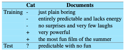
• The prior $P(c)$: $$P(-)=\frac{3}{5} \quad P(+)=\frac{2}{5}$$

The word with doesn’t occur in the training set, so we drop it completely.

The remaining three words are “predictable”, “no”, and “fun”. Their likelihoods from the training set are (with Laplace smoothing):

$$> \begin{aligned} > V=\\{ > \& \text{just, plain, boring, entirely, predictable, and, lacks, energy, no, suprises, very, few, laughs, } \\\\ > \& \text{powerful, the, most, fun, film, of, summer} > \\} > \end{aligned} >$$

$\Rightarrow |V|=20$

The word “predictable” occurs in negative (-) once, therefore, with Laplace smoothing:

$P\left(\text { "predictable" }|-\right) =\frac{1+1}{14+20}$

For the test sentence $S=$ “predictable with no fun”, after removing the word “with”:

$P(-)P(S|-) > P(+)P(S|+)$

$\Rightarrow$ The model predicts the class negative for the test sentence $S$.