HMM Part-of-Speech Tagging
Sequence model/classifier
Assign a label or class to each unit in a sequence
mapping a sequence of observation to a sequence of labels
Hidden Markov Model (HMM) is a probabilistic sequence model
given a sequence of units (words, letters, morphemes, sentences, whatever)
it computes a probability distribution over possible sequences of labels and chooses the best label sequence
Markov Chains
A Markov chain is a model that tells us something about the probabilities of sequences of random variables, states, each of which can take on values from some set. These sets can be words, or tags, or symbols representing anything (E.g., the weather).
💡 A Markov chain makes a very strong assumption that
if we want to predict the future in the sequence, all that matters is the current state.
All the states before the current state have NO impact on the future except via the current state.
- It’s as if to predict tomorrow’s weather you could examine today’s weather but you weren’t allowed to look at yesterday’s weather.
👆 Markov assumption
Consider a sequence of state variables $q_1, q_2, \dots, q_i$
When predicting the future, the past does NOT matter, only the present
$$ P\left(q_{i}=a | q_{1} \ldots q_{i-1}\right)=P\left(q_{i}=a | q_{i-1}\right) $$
Markov chain
embodies the Markov assumption on the probabilities of this sequence
specified by the following components
$Q = q\_1, q\_2, \dots, q\_N$: a set of $N$ states
$A=a\_{11} a\_{12} \dots a\_{n 1} \dots a\_{n n}$: transition probability matrix
- Each $a\_{ij}$ represents the probability of moving from state $i$ to state $j$, s.t. $$ \sum\_{j=1}^{n} a\_{i j}=1 \quad \forall i $$
$\pi=\pi\_{1}, \pi\_{2}, \dots, \pi\_{N}$: an initial probability distribution over states
$\pi_i$: probability that the Markov chain will start in state $i$
Some states $j$ may have $\pi_j = 0$ (meaning that the can NOT be initial states)
$\displaystyle\sum\_{i=1}^{n} \pi\_{i}=1$
Example
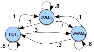
Nodes: states
Edges: transitions, with their probabilities
- The values of arcs leaving a given state must sum to 1.
Setting start distribution $\pi = [0.1, 0.7, 0.2]$ would mean a probability 0.7 of starting in state 2 (cold), probability 0.1 of starting in state 1 (hot), and 0.2 of starting in state 3 (warm)
Hidden Markov Model (HMM)
A Markov chain is useful when we need to compute a probability for a sequence of observable events.
In many cases, however, the events we are interested in are hidden: we don’t observe them directly.
- We do NOT normally observe POS tags in a text
- Rather, we see words, and must infer the tags from the word sequence
$\Rightarrow$ We call the tags hidden because they are NOT observed.
Hidden Markov Model (HMM)
allows us to talk about both observed events (like words that we see in the input) and hidden events (like part-of-speech tags) that we think of as causal factors in our probabilistic model
Specified by:
$Q = {q\_1, q\_2, \dots, q\_N}$: a set of $N$ states
$A=a\_{11} a\_{12} \dots a\_{n 1} \dots a\_{n n}$: transition probability matrix
- Each $a_{ij}$ represents the probability of moving from state $i$ to state $j$, s.t. $$ \sum\_{j=1}^{n} a\_{i j}=1 \quad \forall i $$
$O = {o\_1, o\_2, \dots, o\_T}$: a set of $T$ observations
- Each one drawn from a vocabulary $V = {v_1, v_2, \dots, v_V}$
$B=b\_{i}\left(o\_{t}\right)$: a sequence of observation likelihoods (also called emission probabilities)
- Each expressing the probability of an observation $o\_t$ being generated from a state $q_i$
$\pi=\pi\_{1}, \pi\_{2}, \dots, \pi\_{N}$: an initial probability distribution over states
$\pi\_i$: probability that the Markov chain will start in state $i$
Some states $j$ may have $\pi\_j = 0$ (meaning that the can NOT be initial states)
$\displaystyle\sum_{i=1}^{n} \pi_{i}=1$
A first-order hidden Markov model instantiates two simplifying assumptions
Markov assumption: the probability of a particular state depends only on the previous state
$$ P\left(q\_{i}=a | q\_{1} \ldots q\_{i-1}\right)=P\left(q\_{i}=a | q\_{i-1}\right) $$Output independence: the probability of an output observation $o_i$ depends only on the state that produced the observation $q_i$ and NOT on any other states or any other observations
$$ P\left(o_{i} | q\_{1} \ldots q\_{i}, \ldots, q\_{T}, o\_{1}, \ldots, o\_{i}, \ldots, o\_{T}\right)=P\left(o\_{i} | q\_{i}\right) $$
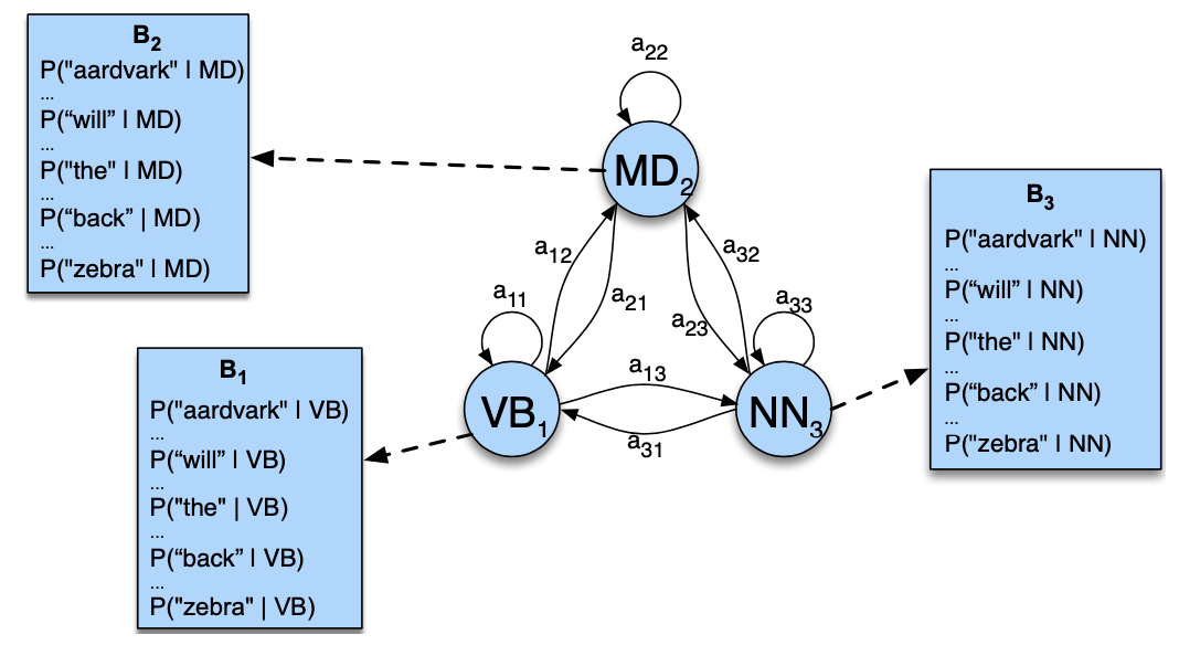
Components of HMM tagger
An HMM has two components, the $A$ and $B$ probabilities
The A probabilities
The $A$ matrix contains the tag transition probabilities $P(t\_i | t\_{i-1})$ which represent the probability of a tag occurring given the previous tag.
- E.g., modal verbs like will are very likely to be followed by a verb in the base form, a VB, like race, so we expect this probability to be high.
We compute the maximum likelihood estimate of this transition probability by counting, out of the times we see the first tag in a labeled corpus, how often the first tag is followed by the second
$$ P\left(t\_{i} | t\_{i-1}\right)=\frac{C\left(t\_{i-1}, t\_{i}\right)}{C\left(t\_{i-1}\right)} $$- For example, in the WSJ corpus, MD occurs 13124 times of which it is followed by VB 10471. Therefore, for an MLE estimate of $$ P(V B | M D)=\frac{C(M D, V B)}{C(M D)}=\frac{10471}{13124}=.80 $$
The B probabilities
The $B$ emission probabilities, $P(w_i|t_i)$, represent the probability, given a tag (say MD), that it will be associated with a given word (say will). The MLE of the emission probability is
$$ P\left(w\_{i} | t\_{i}\right)=\frac{C\left(t\_{i}, w\_{i}\right)}{C\left(t\_{i}\right)} $$- E.g.: Of the 13124 occurrences of MD in the WSJ corpus, it is associated with will 4046 times $$ P(w i l l | M D)=\frac{C(M D, w i l l)}{C(M D)}=\frac{4046}{13124}=.31 $$
Note that this likelihood term is NOT asking “which is the most likely tag for the word will?” That would be the posterior $P(\text{MD}|\text{will})$. Instead, $P(\text{will}|\text{MD})$ answers the question “If we were going to generate a MD, how likely is it that this modal would be will?”
Example: three states HMM POS tagger
HMM tagging as decoding
Decoding: Given as input an HMM $\lambda = (A, B)$ and a sequence of observations $O = o_1, o_2, \dots,o_T$, find the most probable sequence of states $Q = q\_1q\_2 \dots q\_T$
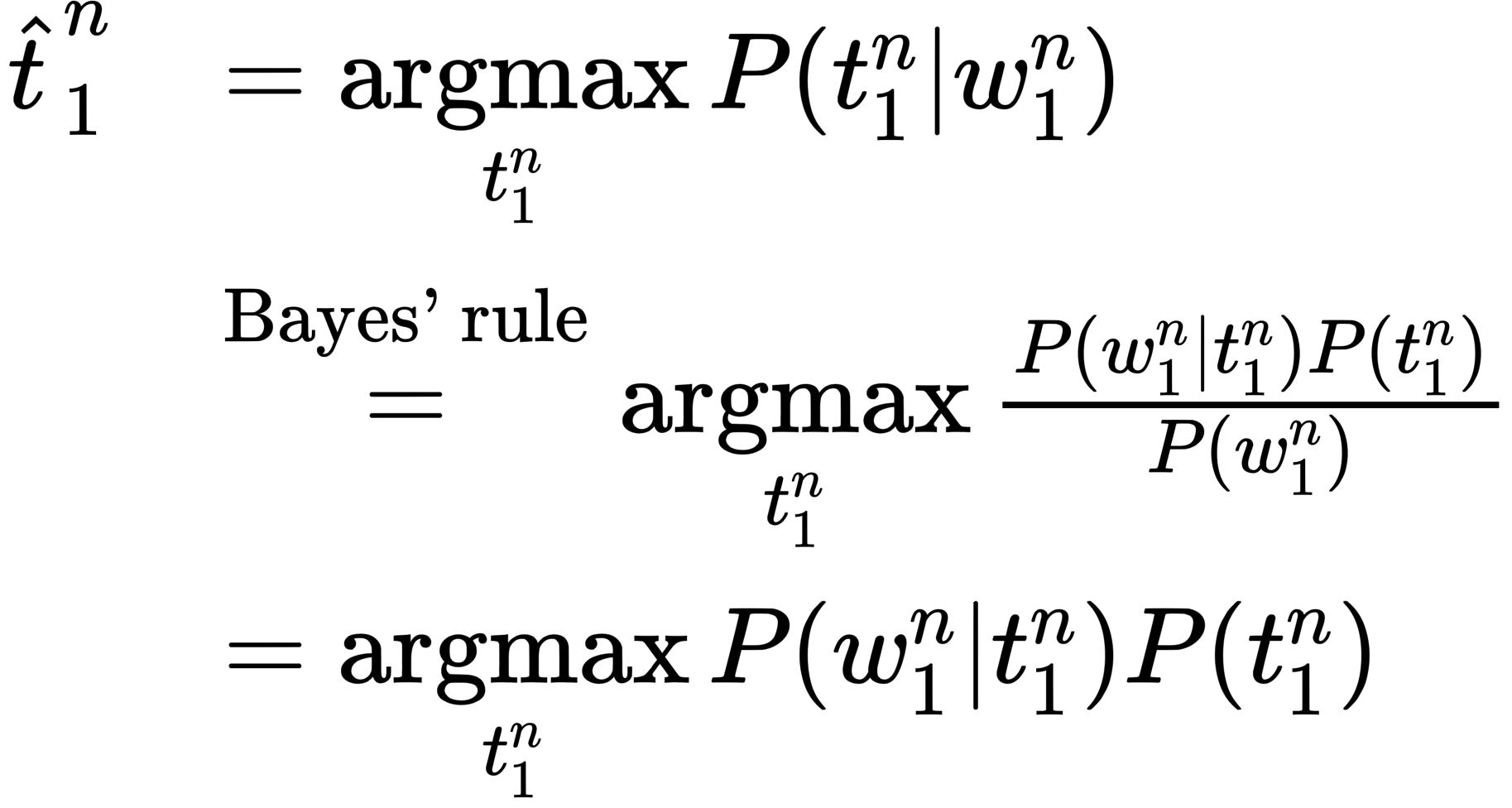
🎯 For part-of-speech tagging, the goal of HMM decoding is to choose the tag sequence $t\_1^n$ that is most probable given the observation sequence of $n$ words $w\_1^n$
HMM taggers make two simplifying assumptions:
the probability of a word appearing depends only on its own tag and is independent of neighboring words and tags
$$ P\left(w\_{1}^{n} | t\_{1}^{n}\right) \approx \prod\_{i=1}^{n} P\left(w\_{i} | t\_{i}\right) $$the probability of a tag is dependent only on the previous tag, rather than the entire tag sequence (the bigram assumption)
$$ P\left(t\_{1}^{n}\right) \approx \prod\_{i=1}^{n} P\left(t\_{i} | t\_{i-1}\right) $$
Combing these two assumptions, the most probable tag sequence from a bigram tagger is:
$$ \hat{t}\_{1}^{n}=\underset{t\_{1}^{n}}{\operatorname{argmax}} P\left(t\_{1}^{n} | w\_{1}^{n}\right) \approx \underset{t\_{1}^{n}}{\operatorname{argmax}} \prod_{i=1}^{n} \overbrace{P\left(w\_{i} | t\_{i}\right)}^{\text {emission}} \cdot \overbrace{P\left(t\_{i} | t\_{i-1}\right)}^{\text{transition }} $$The Viterbi Algorithm
The Viterbi algorithm:
- Decoding algorithm for HMMs
- An instance of dynamic programming
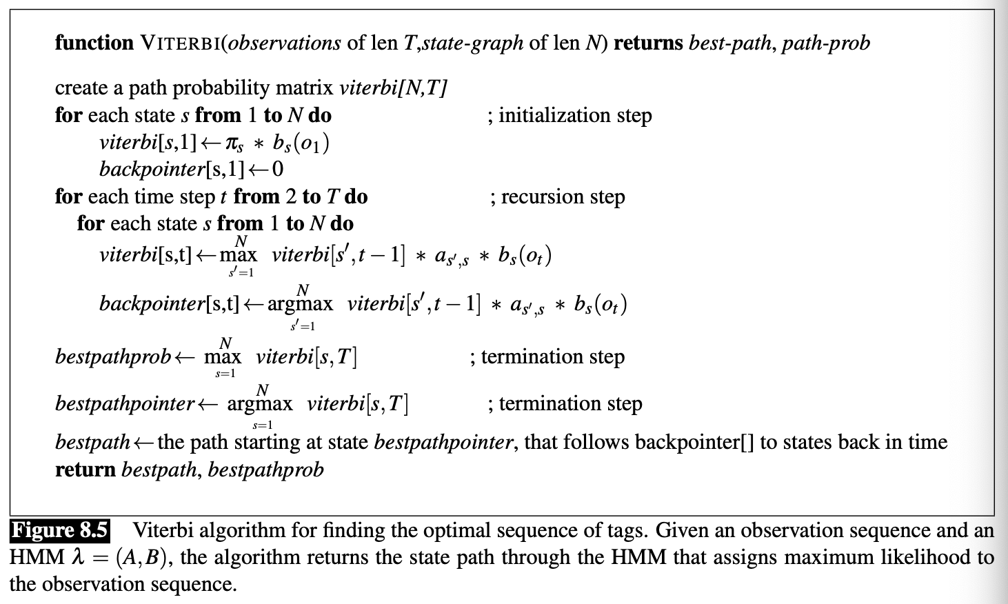
The Viterbi algorithm first sets up a probability matrix or lattice
One column for each observation $o\_t$
One row for each state in the state graph
$\rightarrow$ Each column has a cell for each state $q\_i$ in the single combined automation
Each cell of the lattice $v\_t(j)$
represents the probability that the HMM is in state $j$ after seeing the first $t$ observatins and passing through the most probable state sequence $q\_1, \dots, q\_{t-1}$, given the HMM $\lambda$
The value of each cell $v\_t(j)$ is computed by recursively taking the most probable path that could lead us to this cell
$$ v\_{t}(j)=\max \_{q_{1}, \ldots, q\_{t-1}} P\left(q\_{1} \ldots q\_{t-1}, o\_{1}, o\_{2} \ldots o\_{t}, q\_{t}=j | \lambda\right) $$Represent the most probable path by taking the maximum over all possible previous state sequences $\underset{{q\_{1}, \ldots, q\_{t-1}}}{\max}$
Viterbi fills each cell recursively (like other dynamic programming algorithms)
Given that we had already computed the probability of being in every state at time $t-1$, we compute the Viterbi probability by taking the most probable of the extensions of the paths that lead to the current cell.
For a given state $q_j$ at time $t$, the value $v_t(j)$ is computed as
$$ v\_{t}(j)=\max \_{i=1}^{N} v\_{t-1}(i) a\_{i j} b\_{j}\left(o\_{t}\right) $$- $v\_{t-1}(i)$: the previous Viterbi path probability from the previous time step
- $a\_{ij}$: the transition probability from previous state $q_i$ to current state $q_j$
- $b\_j(o\_t)$: the state observation likelihood of the observation symbol $o_t$ given the current state $j$
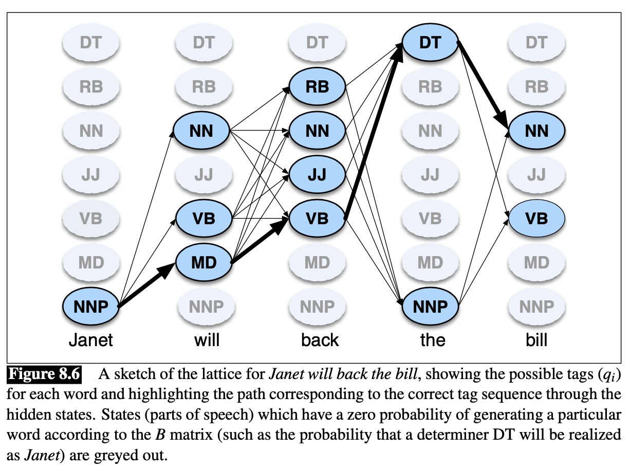
Example 1
Tag the sentence “Janet will back the bill”
🎯 Goal: correct series of tags (Janet/NNP will/MD back/VB the/DT bill/NN)
HMM is defiend by two tables
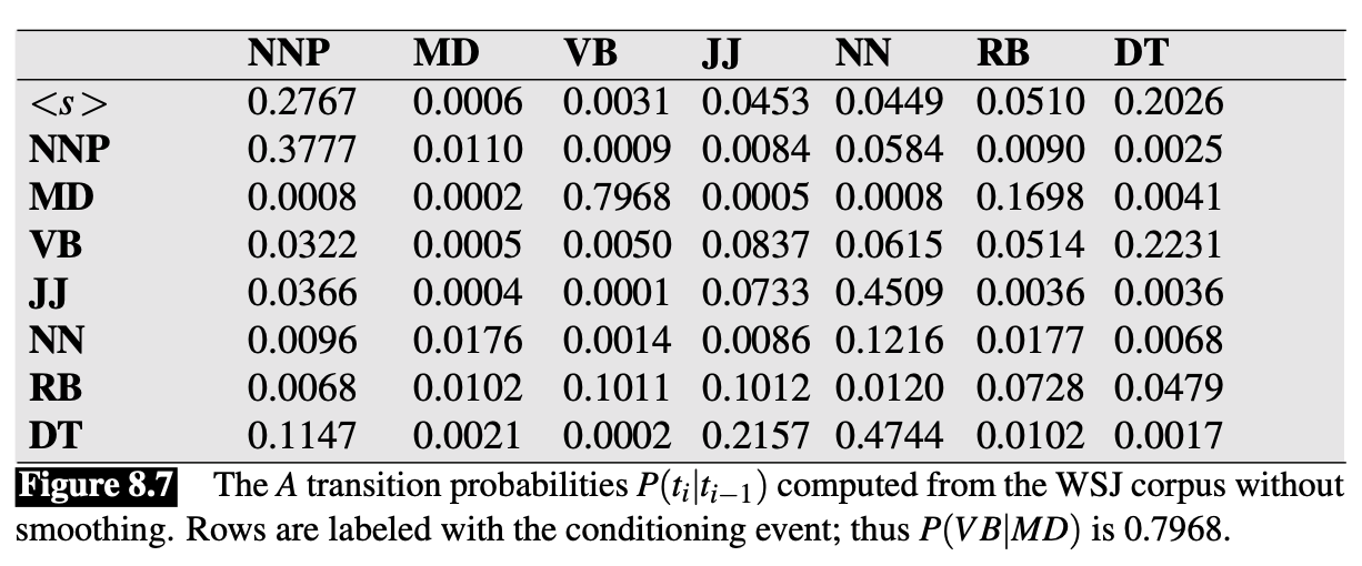
- 👆 Lists the $a\_{ij}$ probabilities for transitioning betweeen the hidden states (POS tags)
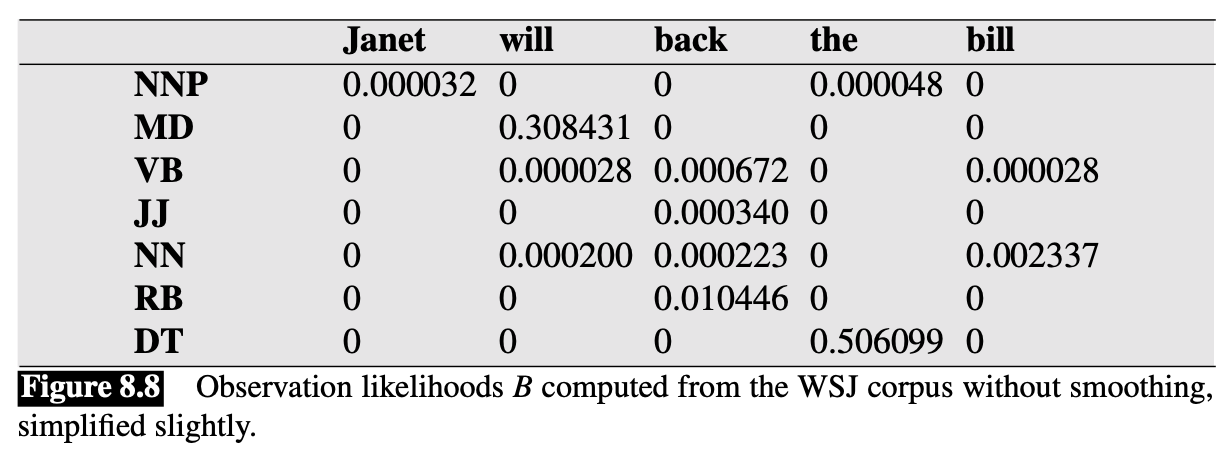
- 👆 Expresses the $b\_i(o\_t)$ probabilities, the observation likelihood s of words given tags
- This table is (slightly simplified) from counts in WSJ corpus
Computation:
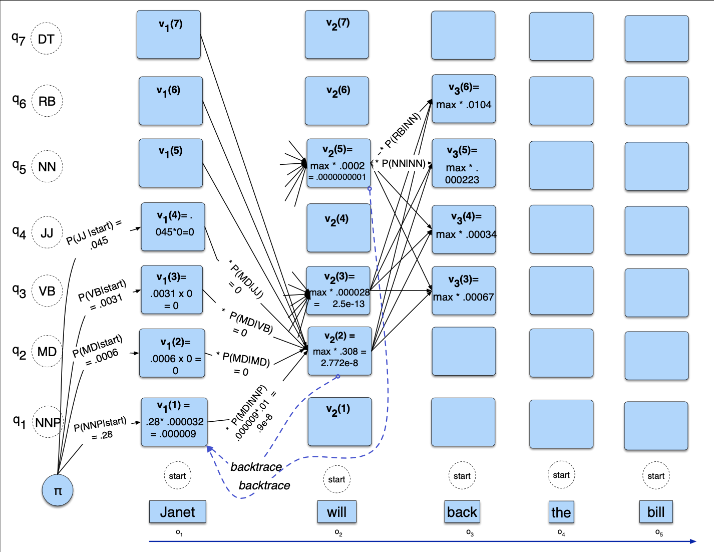
- There’re $N=5$ state columns
- begin in column 1 (for the word Janet) by setting the Viterbi value in each cell to the product of
- the $\pi$ transistion probability (the start probability for that state $i$, which we get from the <s> entry), and
- the observation likelihood of the word Janet givne the tag for that cell
- Most of the cells in the column are zero since the word Janet cannot be any of those tags (See Figure 8.8 above)
- Next, each cell in the will column gets update
- For each state, we compute the value $viterbi[s, t]$ by taking the maximum over the extensions of all the paths from the previous column that lead to the current cell
- Each cell gets the max of the 7 values from the previous column, multiplied by the appropriate transition probability
- Most of them are zero from the previous column in this case
- The remaining value is multiplied by the relevant observation probability, and the (trivial) max is taken. (In this case the final value, 2.772e-8, comes from the NNP state at the previous column. )
Example 2
HMM : Viterbi algorithm - a toy example 👍
Extending the HMM Algorithm to Trigrams
In simple HMM model described above, the probability of a tag depends only on the previous tag
$$ P\left(t_{1}^{n}\right) \approx \prod_{i=1}^{n} P\left(\left.t_{i}\right|_{i-1}\right) $$In practice we use more of the history, letting the probability of a tag depend on the two previous tags
$$ P\left(t_{1}^{n}\right) \approx \prod_{i=1}^{n} P\left(t_{i} | t_{i-1}, t_{i-2}\right) $$- Small increase in performance (perhaps a half point)
- But conditioning on two previous tags instead of one requires a significant change to the Viterbi algorithm 🤪
- For each cell, instead of taking a max over transitions from each cell in the previous column, we have to take a max over paths through the cells in the previous two columns
- thus considering $N^2$ rather than $N$ hidden states at every observation.
In addition to increasing the context window, HMM taggers have a number of other advanced features
let the tagger know the location of the end of the sentence by adding dependence on an end-of-sequence marker for $t_{n+1}$
$$ \hat{t}_{1}^{n}=\underset{t_{1}^{n}}{\operatorname{argmax}} P\left(t_{1}^{n} | w_{1}^{n}\right) \approx \underset{t_{1}^{n}}{\operatorname{argmax}}\left[\prod_{i=1}^{n} P\left(w_{i} | t_{i}\right) P\left(t_{i} | t_{i-1}, t_{i-2}\right)\right] \color{blue}{P\left(t_{n+1} | t_{n}\right)} $$- Three of the tags ($t_{-1}, t_0, t_{n+1}$) used in the context will fall off the edge of the sentence, and hence will not match regular words
- These tags can all be set to be a single special ‘sentence boundary’ tag that is added to the tagset, which assumes sentences boundaries have already been marked.
- Three of the tags ($t_{-1}, t_0, t_{n+1}$) used in the context will fall off the edge of the sentence, and hence will not match regular words
🔴 Problem with trigram taggers: data sparsity
Any particular sequence of tags $t_{i-2}, t_{i-1}, t_{i}$ that occurs in the test set may simply never have occurred in the training set.
Therefore we can NOT compute the tag trigram probability just by the maximum likelihood estimate from counts, following
$$ P\left(t_{i} | t_{i-1}, t_{i-2}\right)=\frac{C\left(t_{i-2}, t_{i-1}, t_{i}\right)}{C\left(t_{i-2}, t_{i-1}\right)} $$- Many of these counts will be zero in any training set, and we will incorrectly predict that a given tag sequence will never occur!
We need a way to estimate $P(t_i|t_{i-1}, t_{i-2})$ even if the sequence $t_{i-2}, t_{i-1}, t_i$ never occurs in the training data
Standard approach: estimate the probability by combining more robust, but weaker estimators.
E.g., if we’ve never seen the tag sequence PRP VB TO, and so can’t compute $P(\mathrm{TO} | \mathrm{PRP}, \mathrm{VB})$ from this frequency, we still could rely on the bigram probability $P(\mathrm{TO} | \mathrm{VB})$, or even the unigram probability $P(\mathrm{TO})$.
The maximum likelihood estimation of each of these probabilities can be computed from a corpus with the following counts:
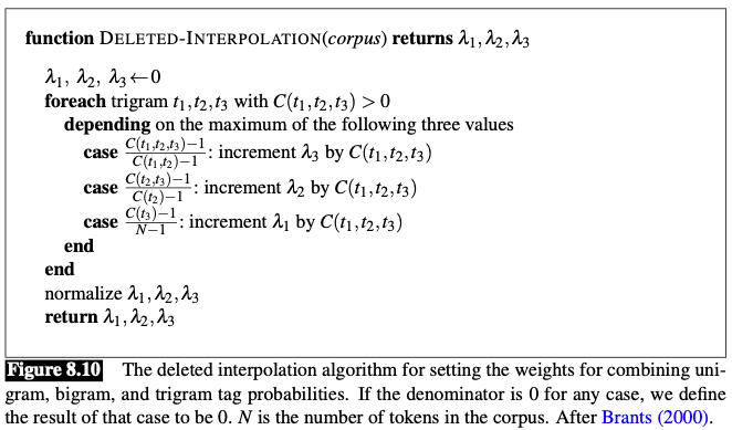
$$ \begin{aligned} \text { Trigrams } \qquad \hat{P}\left(t_{i} | t_{i-1}, t_{i-2}\right) &=\frac{C\left(t_{i-2}, t_{i-1}, t_{i}\right)}{C\left(t_{i-2}, t_{i-1}\right)} \\\\ \text { Bigrams } \qquad \hat{P}\left(t_{i} | t_{i-1}\right) &=\frac{C\left(t_{i-1}, t_{i}\right)}{C\left(t_{i-1}\right)} \\\\ \text { Unigrams } \qquad \hat{P}\left(t_{i}\right)&=\frac{C\left(t_{i}\right)}{N} \end{aligned} $$We use linear interpolation to combine these three estimators to estimate the trigram probability $P\left(t_{i} | t_{i-1}, t_{i-2}\right)$. We estimate the probablity $P\left(t_{i} | t_{i-1}, t_{i-2}\right)$ by a weighted sum of the unigram, bigram, and trigram probabilities
$$ P\left(t_{i} | t_{i-1} t_{i-2}\right)=\lambda_{3} \hat{P}\left(\left.t_{i}\right|_{i-1} t_{i-2}\right)+\lambda_{2} \hat{P}\left(t_{i} | t_{i-1}\right)+\lambda_{1} \hat{P}\left(t_{i}\right) $$- $\lambda_1 + \lambda_2 + \lambda_3 = 1$
- $\lambda$s are set by deleted interpolation
- successively delete each trigram from the training corpus and choose the λs so as to maximize the likelihood of the rest of the corpus.
- helps to set the λs in such a way as to generalize to unseen data and not overfit 👍
- successively delete each trigram from the training corpus and choose the λs so as to maximize the likelihood of the rest of the corpus.
Beam Search
Problem of vanilla Viterbi algorithms
- Slow, when the number of states grows very large
- Complexity: $O(N^2T)$
- $N$: Number of states
- Can be large for trigram taggers
- E.g.: Considering very previous pair of the 45 tags resulting in $45^3=91125$ computations per column!!! 😱
- can be even larger for other applications of Viterbi (E.g., decoding in neural networks)
- Can be large for trigram taggers
- $N$: Number of states
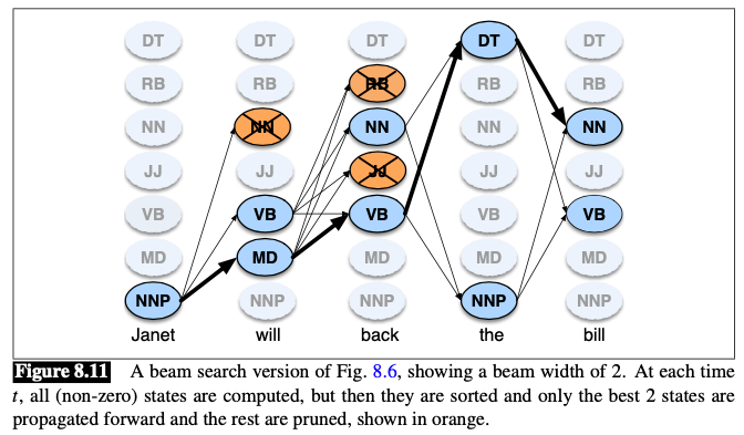
🔧 Common solution: beam search decoding
💡 Instead of keeping the entire column of states at each time point $t$, we just keep the best few hypothesis at that point.
At time $t$:
- Compute the Viterbi score for each of the $N$ cells
- Sort the scores
- Keep only the best-scoring states. The rest are pruned out and NOT continued forward to time $t+1$
Implementation
Keep a fixed number of states (beam width) $\beta$ instead of all $N$ current states
Alternatively $\beta$ can be modeled as a fixed percentage of the $N$ states, or as a probability threshold
Unknown Words
One useful feature for distinguishing parts of speech is word shape
- words starting with capital letters are likely to be proper nouns (NNP).
Strongest source of information for guessing the part-of-speech of unknown words: morphology
Words ending in -s $\Rightarrow$ plural nouns (NNS)
words ending with -ed $\Rightarrow$ past participles (VBN)
words ending with -able $\Rightarrow$ adjectives (JJ)
…
We store for each suffixes of up to 10 letters the statistics of the tag it was associated with in training. We are thus computing for each suffix of length $i$ the probability of the tag $t_i$ given the suffix letters
$$ P\left(t_{i} | l_{n-i+1} \ldots l_{n}\right) $$Back-off is used to smooth these probabilities with successively shorter suffixes.
Unknown words are unlikely to be closed-class words (like prepositions), suffix probabilites can be computed only for words whose training set frequency is $\leq 10$, or only for open-class words.
As $P\left(t_{i} | l_{n-i+1} \ldots l_{n}\right)$ gives a posterior estimate $p(t_i|w_i)$, we can compute the likelihood $p(w_i|t_i)$ tha HMMs require by using Bayesian inversion (i.e., using Bayes’ rule and computation of the two priors $P(t_i)$ and $P(t_i|l_{n-i+1}\dots l_n)$).