The Mechanics of Learning

import torch

Learning is just parameter estimation

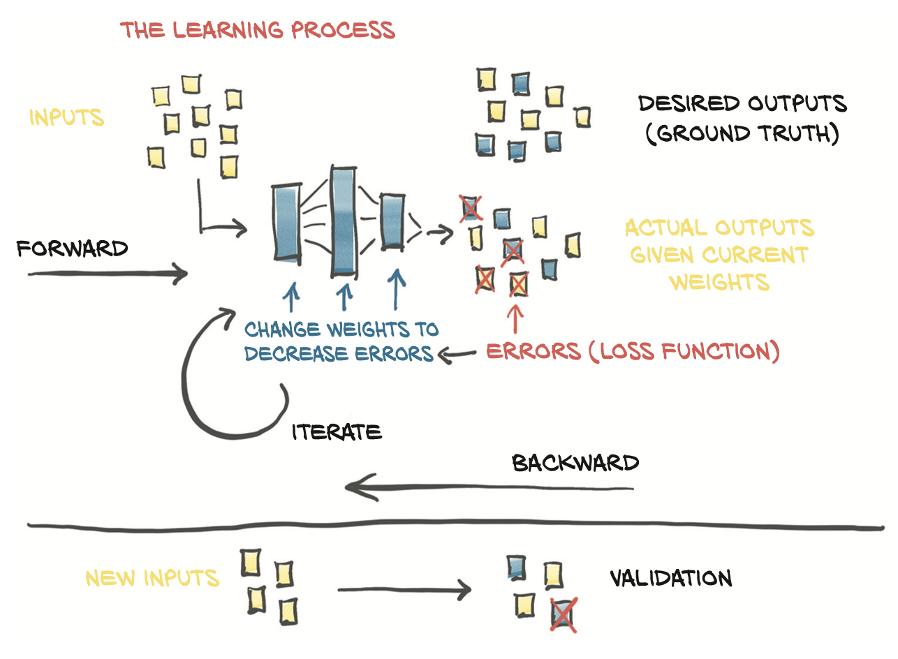
• Given
  • input data
  • corresponding desired outputs (ground truth)
  • initial values for the weights
• The model is fed input data (forward pass)
• A measure of the error is evaluated by comparing the resulting outputs to the ground truth
• In order to optimize the parameter of the model (its weights)
  • The change in the error following a unit change in weights (that is, the gradient of the error with respect to the parameters) is computed using the chain rule for the derivative of a composite function (backward pass)
  • The value of the weights is then updated in the direction that leads to a decrease in the error
  • The procedure is repeated until the error, evaluated on unseen data, falls below an acceptable level.

A simple linear model

t_c = w * t_u + b

• w: weight, tells us how much a given input influence the outputs.
• b: bias, tells us what the output would be if inputs were zero.

Now we need to estimate w and b, the parameters in our model, based on the data we have. We must do it so that temperatures we obtain from running the unknown temperatures t_u through the model are close to temperatures we actually measured in Celsius (t_c). That sounds like fitting a line through a set of measurements!

Let’s flesh it out again:

• we have a model with some unknown parameters, and we need to estimate those parameters so that the error between predicted outputs and measured values is as low as possible.
• We need to exactly define a measure of the error. Such a measure, which we refer to as the loss function, should be high if the error is high and should ideally be as low as possible for a perfect match.
• Our optimization process should therefore aim at finding w and b so that the loss function is at a minimum.

Modeling with PyTorch

We can define the model as a python function:

def model(t_u, w, b):
    """
    t_u: input tensor
    w: weight parameter
    b: bias parameter
    """
    return w * t_u + b

For loss function we choose Mean Square Loss (building a tensor of differences, taking their square element-wise, and finally producing a scalar loss function by averaging all of the elements in the resulting tensor):

def loss_fn(t_p,t_c):
    squared_diffs = (t_p - t_c) ** 2
    return squared_diffs.mean()

Down along the gradient

We’ll optimize the loss function with respect to the parameters using the gradient descent algorithm, which is actually a very simple idea and scales up surprisingly well to large neural network models with mil- lions of parameters.

params -= learning_rate * params.grad

PyTorch’s autograd

PyTorch provides a mechanisam called autograd: PyTorch tensors can remember where they come from, in terms of the operations and parent tensors that originated them, and they can automatically provide the chain of derivatives of such operations with respect to their inputs. This means

• we won’t need to derive our model by hand 👏
• given a forward expression, no matter how nested, PyTorch will automatically provide the gradient of that expression with respect to its input parameters 👏

Applying autograd

In order to activate autograd, we need to initialize the parameters tensor with requires_grad=True

params = torch.tensor([1.0, 0.0], requires_grad=True)

Using the grad attribute

requires_grad=True is telling PyTorch to track the entire family tree of tensors resulting from operations on params. In other words, any tensor that will have params as an ancestor will have access to the chain of functions that were called to get from params to that tensor. In case these functions are differentiable (and most PyTorch tensor operations will be), the value of the derivative will be automatically populated as a grad attribute of the params tensor.

In general, all PyTorch tensors have an attribute named grad. Normally, it’s None at the beginning:

params.grad is None

True=

All we have to do to populate it is to start with a tensor with requires_grad set to True, then call the model and compute the loss, and then call backward() on the loss tensor:

loss = loss_fn(model(t_u, *params), t_c)
loss.backward()

At this point, the grad attribute of params contains the derivatives of the loss with respect to each element of params.

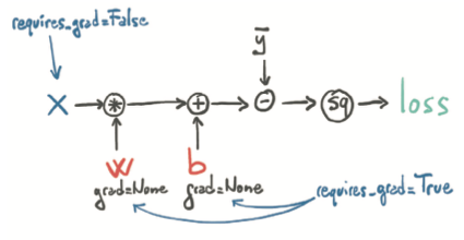
What happened under the hood?

When we compute our loss while the parameters w and b require gradients, in addition to performing the actual computation, PyTorch creates the autograd graph with the operations (in black circles) as nodes:

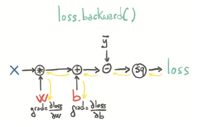
When we call loss.backward(), PyTorch traverses this graph in the reverse direction to compute the gradients:

if params.grad is not None:
    params.grad.zero_()

Now our autograd-enabled training code looks like this:

def training_loop(n_epochs, learning_rate, params, t_u, t_c):
    for epoch in range(1, n_epochs + 1):
        if params.grad is not None:
            params.grad.zero_()

        # forward pass
        t_p = model(t_u, *params)

        # backward pass
        loss = loss_fn(t_p, t_c)
        loss.backward()

        # update params
        with torch.no_grad():
            params -= learning_rate * params.grad
        
        # logging
        if epoch % 500 == 0:
            print('Epoch %d, Loss %f' % (epoch, float(loss)))

    return params

PyTorch’s optimizers

There are several optimization strategies and tricks that can assist convergence, especially when models get complicated. The torch module has an optim submodule where we can find classes implementing different optimization algorithms.

import torch.optim as optim

dir(optim)

['ASGD',
 'Adadelta',
 'Adagrad',
 'Adam',
 'AdamW',
 'Adamax',
 'LBFGS',
 'Optimizer',
 'RMSprop',
 'Rprop',
 'SGD',
 'SparseAdam',
 '__builtins__',
 '__cached__',
 '__doc__',
 '__file__',
 '__loader__',
 '__name__',
 '__package__',
 '__path__',
 '__spec__',
 'lr_scheduler']

Every optimizer constructor takes a list of parameters (aka PyTorch tensors, typically with requires_grad set to True) as the first input. All parameters passed to the optimizer are retained inside the optimizer object so the optimizer can update their values and access their grad attribute:

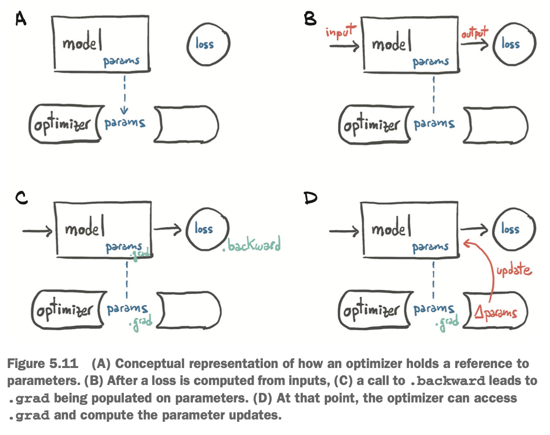
Each optimizer exposes two methods

• zero_grad: zeroes the grad attribute of all the parameters passed to the optimizer upon construction.

• step: updates the value of those parameters according to the optimization strategy implemented by the specific optimizer.

Let’s apply optimizer to our training loop:

# initialize parameters
params = torch.tensor([1.0, 0.0], requires_grad=True)

# choose learning rate and optimizer
learning_rate = 1e-2
optimizer = optim.SGD([params], lr=learning_rate)

def training_loop(n_epochs, optimizer, params, t_u, t_c):
    for epoch in range(1, n_epochs+1):
        t_p = model(t_u, *params)
        loss = loss_fn(t_p, t_c)
				
        # zero_grad before backward!
        optimizer.zero_grad()
        
        loss.backward()

        # # update params
        optimizer.step()

        if epoch % 500 == 0:
            print(f'Epoch: {epoch}, loss: {float(loss)}')

    return params

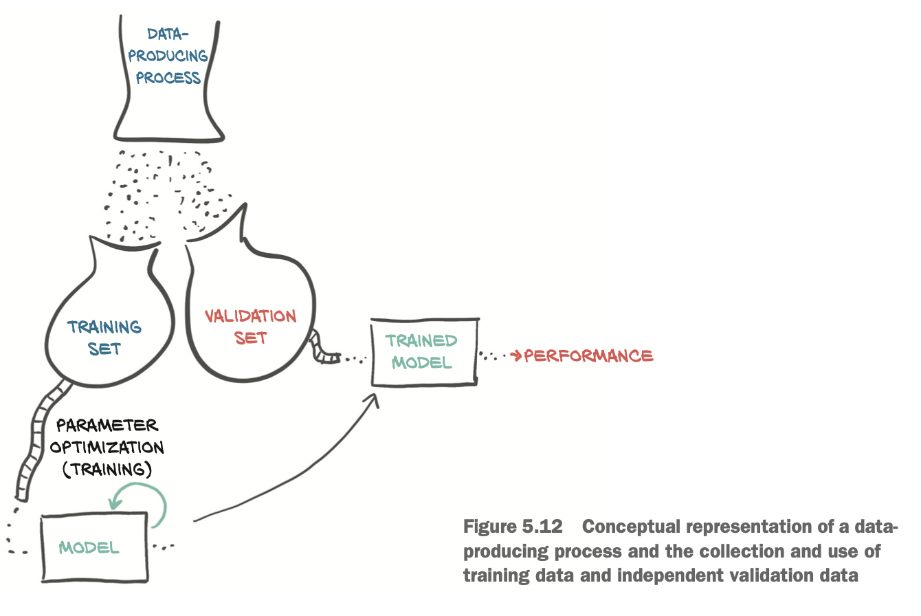
Training, validation, and overfitting

A highly adaptable model will tend to use its many parameters to make sure the loss is minimal at the data points, but we’ll have no guarantee that the model behaves well away from or in between the data points. 🤪

Overfitting: Evaluating the loss at independent data points yield higher-than-expected loss.

To overcome overfitting,

• we must take a few data points out of our dataset (the validation set) and only fit our model on the remaining data points (the training set).
• while we’re fitting the model, we can evaluate the loss once on the training set and once on the validation set.
• When we’re trying to decide if we’ve done a good job of fitting our model to the data, we must look at both!

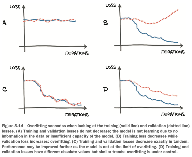
Evaluating the training loss

If the training loss is not decreasing, there may be two possibilities:

• the model is too simple for the data
• our data just doesn’t contain meaningful information that lets it explain the output

Generalizing to the validation set

If the training loss and the validation loss diverge, we’re overfitting. Overfitting really looks like a problem of making sure the behavior of the model in between data points is sensible for the process we’re trying to approximate.

How to avoid overfitting?

• Make sure we get enough data for the process

• Make our model simple

  A simpler model may not fit the training data as perfectly as a more complicated model would, but it will likely behave more regularly in between data points.

• Make sure the model that is capable of fitting the training data is as regular as possible in between them.

  • Adding penalization terms to the loss function, to make it cheaper for the model to behave more smoothly and change more slowly (up to a point)
  • Add noise to the input samples, to artificially create new data points in between training data samples and force the model to try to fit those, too.

We’ve got some nice trade-offs:

• we need the model to have enough capacity for it to fit the training set.
• we need the model to avoid overfitting

Therefore, in order to choose the right size for a neural network model in terms of parameters, the process is based on two steps:

1. increase the size until it fits,
2. then scale it down until it stops overfitting.

Splitting a dataset

Use PyTorch’s randperm function

randperm function: Shuffle the elements of a tensor amounts to finding a permutation of its indices.

n_samples = t_u.shape[0]
n_val = int(0.2 * n_samples)

shuffled_indices = torch.randperm(n_samples)

train_indices = shuffled_indices[:-n_val]
val_indices = shuffled_indices[-n_val:]

# training set
train_t_u = t_u[train_indices]
train_t_c = t_c[train_indices]

# validation set
val_t_u = t_u[val_indices]
val_t_c = t_c[val_indices]

Our training loop doesn’t really change. We just want to additionally evaluate the validation loss at every epoch, to have a chance to recognize whether we’re overfitting:

def training_loop(n_epochs, optimizer, params, train_t_u, val_t_u,
                  train_t_c, val_t_c):
    for epoch in range(1, n_epochs + 1):
        train_t_p = model(train_t_u, *params)

        train_loss = loss_fn(train_t_p, train_t_c)

        val_t_p = model(val_t_u, *params)
        val_loss = loss_fn(val_t_p, val_t_c)

        optimizer.zero_grad()
        train_loss.backward()
        optimizer.step()

        if epoch <= 3 or epoch % 500 == 0:
            print(f"Epoch {epoch}, Training loss {train_loss.item():.4f},"
                  f" Validation loss {val_loss.item():.4f}")

    return params

Observing the training

Our main goal: both the training loss and the validation loss decreasing. While ideally both losses would be roughly the same value, as long as the validation loss stays reasonably close to the training loss, we know that our model is continuing to learn generalized things about our data.

Switching autograd off for validation

We only ever call backward on train_loss and errors will only ever backpropagate based on the training set. The validation set is used to provide an independent evaluation of the accuracy of the model’s output on data that wasn’t used for training.

Since we’re not ever calling backward on val_loss, we could in fact just call model and loss_fn as plain functions, without tracking the computation. PyTorch allows us to switch off autograd when we don’t need it, using the torch.no_grad context manager.

def training_loop(n_epochs, optimizer, params, train_t_u, val_t_u,
                  train_t_c, val_t_c):
    for epoch in range(1, n_epochs + 1):
        train_t_p = model(train_t_u, *params)

        train_loss = loss_fn(train_t_p, train_t_c)

        with torch.no_grad():
            val_t_p = model(val_t_u, *params)
            val_loss = loss_fn(val_t_p, val_t_c)

            # Checks that our output requires_grad args are 
            # forced to False inside this block
            assert val_loss.requires_grad == False

        optimizer.zero_grad()
        train_loss.backward()
        optimizer.step()

        if epoch <= 3 or epoch % 500 == 0:
            print(f"Epoch {epoch}, Training loss {train_loss.item():.4f},"
                  f" Validation loss {val_loss.item():.4f}")

    return params

Run with autograd enabled or disabled

Using the related set_grad_enabled context, we can also condition the code to run with autograd enabled or disabled, according to a Boolean expression—typically indicating whether we are running in training or inference mode.

For instance, we could define a calc_forward function that takes data as input and runs model and loss_fn with or without autograd according to a Boolean is_train argument:

def cal_forward(t_u, t_c, is_train):
    with torch.set_grad_enabled(is_train):
        t_p = model(t_u, *params)
        loss = loss_fn(t_p, t_c)

    return loss