Learning from Images

Dataset of images

torchvision module:

• automatically download the dataset

• load it as a collection of PyTorch tensors

• For example, download CIFAR-10 dataset:

  from torchvision import datasets
  
  data_path = '../data-unversioned/p1ch7/' # root directory
  
  # Instantiates a dataset for the training data; 
  # TorchVision downloads the data if it is not present.
  cifar10 = datasets.CIFAR10(data_path, train=True, download=True)
  
  # With train=False, this gets us a dataset for the validation data
  cifar10_val = datasets.CIFAR10(data_path, train=False, download=True) 
  

dataset submodule:

• gives us precanned access to the most popular computer vision datasets, such as MNIST, Fashion-MNIST, CIFAR-100, SVHN, Coco, and Omniglot.
• In each case, the dataset is returned as a subclass of torch.utils.data.Dataset.

Dataset class

torch.utils.data.Dataset:

• Concept: does NOT necessarily hold the data, but provides uniform access to it through __len__ and __getitem__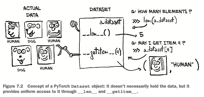

  

• is an object that is required to implement two methods:

  • __len__: returns the number of items in the dataset
  • __getitem__: returns the item, consisting of a smaple and its corresponding label (an integer index)

Dataset transformations

torchvision.transforms

• defines a set of composable, function-like objects that can be passed as an argument to a torchvision dataset

  from torchvision import transforms
  
  dir(transforms)
  

  ['CenterCrop',
   'ColorJitter',
   'Compose',
   'ConvertImageDtype',
   'FiveCrop',
   'Grayscale',
   'Lambda',
   'LinearTransformation',
   'Normalize',
   'PILToTensor',
   'Pad',
   'RandomAffine',
   'RandomApply',
   'RandomChoice',
   'RandomCrop',
   'RandomErasing',
   'RandomGrayscale',
   'RandomHorizontalFlip',
   'RandomOrder',
   'RandomPerspective',
   'RandomResizedCrop',
   'RandomRotation',
   'RandomSizedCrop',
   'RandomVerticalFlip',
   'Resize',
   'Scale',
   'TenCrop',
   'ToPILImage',
   'ToTensor',
   '__builtins__',
   '__cached__',
   '__doc__',
   '__file__',
   '__loader__',
   '__name__',
   '__package__',
   '__path__',
   '__spec__',
   'functional',
   'functional_pil',
   'functional_tensor',
   'transforms']
  

• perform transformations on the data after it is loaded but before it is returned by __getitem__.

ToTensor

• turns NumPy arrays and PIL images to tensors.

• also takes care to lay out the dimensions of the output tensor as C × H × W

• Once instantiated, it can be called like a function with the PIL image as the argument, returning a tensor as output

  from torchvision import transforms
  
  to_tensor = transforms.ToTensor()
  img_t = to_tensor(img)
  

We can pass the transform dierctly as an argument to dataset instructor:

tensor_cifar10 = datasets.CIFAR10(data_path, train=True, download=False, 
                                  transform=transforms.ToTensor())

• At this point, accessing an element of the dataset will return a tensor, rather than a PIL image

  img_t, _ = tensor_cifar10[99]
  type(img_t)
  

  torch.Tensor
  

• Whereas the values in the original PIL image ranged from 0 to 255 (8 bits per channel), the ToTensor transform turns the data into a 32-bit floating-point per channel, scaling the values down from 0.0 to 1.0.

  img_t.min(), img_t.max()
  

  (tensor(0.), tensor(1.))
  

Normalizing data

We can chain transforms using transforms.Compose, and they can handle normalization and data augmentation transparently, directly in the data loader. It’s good practice to normalize the dataset so that each channel has zero mean and unitary standard deviation. Also, normalizing each channel so that it has the same distribution will ensure that channel information can be mixed and updated through gradient descent using the same learning rate.

transforms.Normalize: compute the mean value and the standard deviation of each channel across the dataset and apply the following transform: v_n[c] = (v[c] - mean[c]) / stdev[c].

Steps for normalization:

1. Stack all the tensors returned by the dataset along an extra dimension

   imgs = torch.stack([img_t for img_t, _ in tensor_cifar10], dim=3)
   imgs.shape
   

   torch.Size([3, 32, 32, 50000])
   

   (Channels x Height x Width x #images)

2. Compute mean and standard derivation per channel:

   • Mean

     # Recall that view(3, -1) keeps the three channels and 
     # merges all the remaining dimensions into one, figuring out the appropriate size. 
     # Here our 3 × 32 × 32 image is transformed into a 3 × 1,024 vector, 
     # and then the mean is taken over the 1,024 elements of each channel.
     imgs.view(3, -1).mean(dim=1)
     

     tensor([0.4915, 0.4823, 0.4468])
     

   • Standard derivation

     imgs.view(3, -1).std(dim=1)
     

     tensor([0.2470, 0.2435, 0.2616])
     

3. Initialize the Normalize transform and chain it in transforms.Compose

   transforms.Normalize((0.4915, 0.4823, 0.4468), (0.2470, 0.2435, 0.2616))
   
   transform = transforms.Compose([transforms.ToTensor(),
                                   transforms.Normalize((0.4915, 0.4823, 0.4468), 
                                                        (0.247, 0.2435, 0.2616))])
   
   transformed_cifar10 = datasets.CIFAR10(data_path, train=True, download=False,
                                        transform=transform)
   

Classifier

Assume that we’ll pick out all the birds and airplanes from our CIFAR-10 dataset and build a neural network that can tell birds and airplanes apart. This is a classification problem.

A fully connected model

An image is just a set of numbers laid out in a spatial configuration. In theory if we just take the image pixels and straighten them into a long 1D vector, we could consider those numbers as input features, which can be illustrated with the following figure:

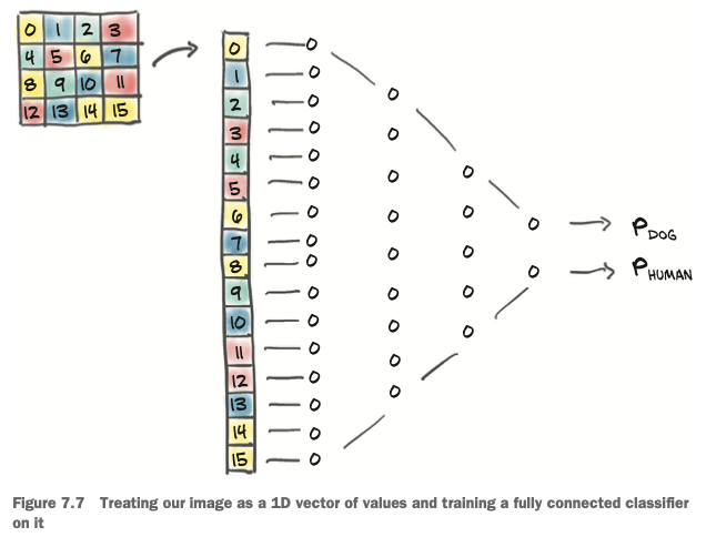
In our case, each image is 32 x 32 x 3, that’s 3072 input features per sample. Let’s build a simple fully connected neural network:

import torch.nn as nn

n_input = 3072
n_hidden = 512 # just arbitrary choice
n_out = 2 # there're 2 classes: bird and airplan

model = nn.Sequential(nn.Linear(n_in, n_hidden),
                    nn.Tanh(),
                    nn.Linear(n_hidden, n_out))

Output of a classifier

We need to recgnize that the output is categorical: it’s either a bird or an airplane.

In the ideal caes, the network would ouput torch.tensor([1.0, 0.0]) for an airplane and torch.tensor([0.0, 1.0]) for a bird. Practically speaking, since our classifier will not be perfect, we can expect the network to output something in between. The key realization in this case is that we can interpret our output as probabilities: the first entry is the probability of “airplane,” and the second is the probability of “bird.”

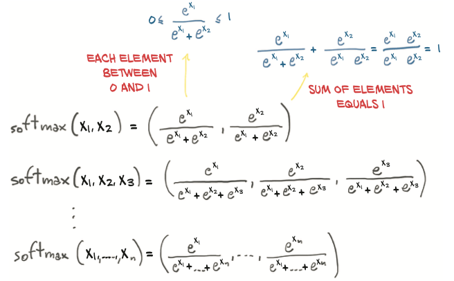
Casting the problem in terms of probabilities imposes a few extra constraints on the outputs of our network:

• Each element of the output must be in the [0.0, 1.0] range (a probability of an outcome cannot be less than 0 or greater than 1).
• The elements of the output must add up to 1.0 (we’re certain that one of the two outcomes will occur).

This is called softmax: we take the elements of the vector, compute the elementwise exponential, and divide each element by the sum of exponentials

In code:

def softmax(x):
    return torch.exp(x) / torch.exp(x).sum()

The nn module makes softmax available as a module, which requires us to specify the dimension along which the softmax function is applied. Now we add a softmax at the end of our model,

model = nn.Sequential(nn.Linear(n_in, n_hidden),
                      nn.Tanh(),
                      nn.Linear(n_hidden, n_out),
                      nn.Softmax(dim=1))

After training, we will be able to get the label as an index by computing the argmax of the output probabilities: that is, the index at which we get the maximum probability. Conveniently, when supplied with a dimension, torch.max returns the maximum element along that dimension as well as the index at which that value occurs.

_, index = torch.max(out, dim=1)

Loss for classifying

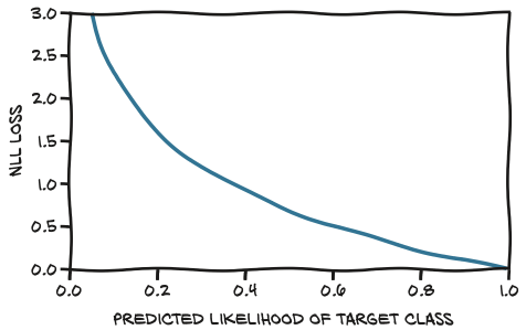
We want to penalize misclassifications. What we need to maximize is the probability associated with the correct class, which is referred to as the likelihood. I.e, we want a loss function that is

• high when the likelihood is low: so low that the alternatives have a higher probability.
• low when the likelihood is higher than the alternatives, and we’re not really fixated on driving the probability up to 1.

A loss function behaves that way is called negative log likelihood (NLL):

PyTorch has an nn.NLLLoss class.

The workaround is to use nn.LogSoftmax instead of nn.Softmax, which takes care to make the calculation numerically stable.

model = nn.Sequential(nn.Linear(n_in, n_hidden),
                     nn.Tanh(),
                     nn.Linear(n_hidden, 2),
                     nn.LogSoftmax(dim=1))

loss = nn.NLLLoss()

# compute the NLL loss for a single sample:
img, label = cifar2[0] # cifar2 is the modified dataset containing only birds and airplanes
out = model(img.view(-1).unsqueeze(0))

loss(out, torch.tensor([label]))

model = nn.Sequential(nn.Linear(n_in, n_hidden),
                     nn.Tanh(),
                     nn.Linear(n_hidden, 2))

loss_fn = nn.CrossEntropyLoss()

Training the classifier

Training the classifier is similar to the process we’ve learned before:

import torch
import torch.nn as nn

model = nn.Sequential(nn.Linear(n_in, n_hidden),
                     nn.Tanh(),
                     nn.Linear(n_hidden, 2))

loss_fn = nn.CrossEntropyLoss()

optimizer = optim.SGD(model.parameters(), lr=learning_rate)

loss_fn = nn.NLLLoss()

n_epochs = 100

for epoch in range(n_epochs):
    for img, label in cifar2:
        # forward
        out = model(img.view(-1).unsqueeze(0))
        loss = loss_fn(out, torch.tensor([label]))
        
        optimizer.zero_grad()

        # backward
        loss.backward()
        
        # update
        optimizer.step()
    print(f'Epoch: {epoch}, Loss: {float(loss):4.3f}')

Data loader

The torch.utils.data module has a class that helps with shuffling and organizing the data in minibatches: DataLoader. The job of a data loader is to sample minibatches from a dataset, giving us the flexibility to choose from different sampling strategies.

A very common strategy is uniform sampling after shuffling the data at each epoch:

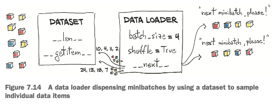
The DataLoader constructor takes a Dataset object as input, along with batch_size and a shuffle Boolean that indicates whether the data needs to be shuffled at the beginning of each epoch:

train_loader = torch.utils.data.DataLoader(cifar2, batch_size=64, shuffle=True) # training set
val_loader = torch.utils.data.DataLoader(cifar2_val, batch_size=64, shuffle=False) # validation set

A DataLoader can be iterated over, so we can use it directly in the inner loop of our new training code:

for epoch in range(n_epochs):
    for imgs, labels in train_loader:
        batch_size = imgs.shape[0]
        outputs = model(imgs.view(batch_size, -1))
        loss = loss_fn(outputs, labels)

        optimizer.zero_grad()
        loss.backward()
        optimizer.step()

    # Due to the shuffling, this now prints the loss for a random batch
    print(f"Epoch: {epoch}, Loss: {float(loss):4.3f}")

Parameters of the model

PyTorch offers a quick way to determine how many parameters a model has through the parameters() method of nn.Model.

To find out how many elements are in each tensor instance, we can call the numel method. Summing those gives us our total count. Depending on our use case, counting parameters might require us to check whether a parameter has requires_grad set to True, as well. We might want to differentiate the number of trainable parameters from the overall model size.

numel_list = [p.numel() for p in model.parameters() if p.requires_grad == True]
sum(numel_list), numel_list

(1574402, [1572864, 512, 1024, 2])

7.2.7 The limits of going fully connected

The model we trained above is like taking every single input value—that is, every single component in our RGB image—and computing a linear combination of it with all the other values for every output feature.

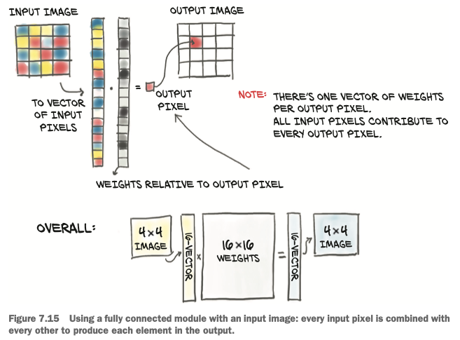
• On one hand, we are allowing for the combination of any pixel with every other pixel in the image being potentially relevant for our task.
• On the other hand, we aren’t utilizing the relative position of neighboring or faraway pixels, since we are treating the image as one big vector of numbers.

The problem of our fully connected network is: it is NOT translation invariant. The solution to our current set of problems is to change our model to use convolutional layers.