Build and Train a Neural Network
Neural networks can be constructed using the torch.nn package.
An nn.Module contains layers, and a method forward(input) that returns the output.
A typical training procedure for a neural network is:
Define the neural network that has some learnable parameters (or weights)
Iterate over a dataset of inputs
Update the weights of the network, typically using a simple update rule:
weight = weight - learning_rate * gradient
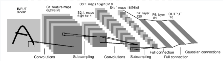
In the following we will take LeNet as example for network construction and see how the procedure works.
Define the Network
import torch
import torch.nn as nn
import torch.nn.functional as F
class Net(nn.Module):

    def __init__(self):
        super(Net, self).__init__()

        # 1 input image channel, 6 output channels, 3x3 convolution kernel
        self.conv1 = nn.Conv2d(1, 6, 3)
        # 6 input image channel, 16 output channels, 3x3 convolution kernel
        self.conv2 = nn.Conv2d(6, 16, 3)

        # Fully connected layer
        # affine operation: y = Wx + b
        self.fc1 = nn.Linear(16 * 6 * 6, 120) # 6*6 from image dimension
        self.fc2 = nn.Linear(120, 84)
        self.fc3 = nn.Linear(84, 10)

    def forward(self, x):

        # Convolution operation
        x = self.conv1(x)
        # ReLU
        x = F.relu(x)
        # Max pooling over a (2, 2) window
        x = F.max_pool2d(x, (2, 2))

        # If the size is a square, we can only specify a single number
        x = F.max_pool2d(F.relu(self.conv2(x)), 2)

        # FC layer
        x = x.view(-1, self.num_flat_features(x)) # flatten
        x = F.relu(self.fc1(x))
        x = F.relu(self.fc2(x))
        x = self.fc3(x)

        return x

    def num_flat_features(self, x):
        size = x.size()[1:] # all dimensions except the batch dimension
        num_features = 1
        for s in size:
            num_features *= s
        return num_features
net = Net()
print(net)
Net(
  (conv1): Conv2d(1, 6, kernel_size=(3, 3), stride=(1, 1))
  (conv2): Conv2d(6, 16, kernel_size=(3, 3), stride=(1, 1))
  (fc1): Linear(in_features=576, out_features=120, bias=True)
  (fc2): Linear(in_features=120, out_features=84, bias=True)
  (fc3): Linear(in_features=84, out_features=10, bias=True)
)
We just have to define the forward function, and the backward function (where gradients are computed) is automatically defined for us using autograd.
we can use any of the Tensor operations in the forward function.
The learnable parameters of a model are returned by net.parameters().
params = list(net.parameters())
Let’s check out the size/number of parameters in the first CONV layer:
(In the first CONV layer there’re 6 filters. Each filter has one channel and the size of 3x3)
print(f"#conv1's weight: {params[0].size()}")
#conv1's weight: torch.Size([6, 1, 3, 3])
Forward
Let’s try a random 32x32 input (expected size of LeNet)
input = torch.randn(1, 1, 32, 32)
out = net(input)
print(out)
tensor([[ 0.0114, 0.1167, -0.0449, -0.0072, -0.0791, -0.0805, -0.0467, 0.0667, -0.0750, 0.0985]], grad_fn=<AddmmBackward>)
Backward
Zero the gradient buffers of all parameters and backprops with random gradients
net.zero_grad()
out.backward(torch.randn(1, 10))
Note that torch,nn ONLY supports mini-batches. The entire torch.nn package only supports inputs that are a mini-batch of samples, and NOT a single sample.
For example, nn.Conv2d will take in a 4D Tensor of nSamples x nChannels x Height x Width.
For a single sample, just use input.unsqueeze(0) to add a fake batch dimension.
Loss Function
A loss function takes the (output, target) pair of inputs, and computes a value that estimates how far away the output is from the target.
output = net(input)
target = torch.randn(10) # dummy target
target = target.view(1, -1) # make it the same shape as output
criterion = nn.MSELoss() # here we use Mean Squared Error as our loss function

loss = criterion(output, target) # Compute loss
If we follow loss in the backward direction, using its .grad_fn attribute, we will see a computational graph looks like this:
input -> conv2d -> relu -> maxpool2d
      -> conv2d -> relu -> maxpool2d
      -> view -> linear -> relu -> linear -> relu -> linear
      -> MSELoss
      -> loss
So, when we call loss.backward(), the whole graph is differentiated w.r.t. the loss, and all Tensors in the graph that has requires_grad=True will have their .grad Tensor accumulated with the gradient.
Backpropagation
To backpropagate the error all we have to do is to loss.backward(). Remember that we need to clear the existing gradients though, else gradients will be accumulated to existing gradients.
net.zero_grad() # zeroes the gradient buffers of all parameters

print('conv1.bias.grad before backward:')
print(net.conv1.bias.grad)

loss.backward(retain_graph=True)

print('conv1.bias.grad after backward:')
print(net.conv1.bias.grad)
conv1.bias.grad before backward:
tensor([0., 0., 0., 0., 0., 0.])
conv1.bias.grad after backward:
tensor([-0.0037,  0.0082,  0.0034, -0.0042,  0.0045, -0.0054])
Update Weights
The simplest update rule used in practice is the Stochastic Gradient Descent (SGD):
weight = weight - learning_rate * gradient
There’re various different update rules such as SGD, Nesterov-SGD, Adam, RMSProp, etc. Package torch.optim implements all these methods.
import torch.optim as optim

# Specify optimizer
optimizer = optim.SGD(net.parameters(), lr=0.01)

# In training loop:
# 1. Zero the gradient buffer
optimizer.zero_grad()

# 2. Forward propagation throught the neural network and get output
output = net(input)

# 3. Compute loss
loss = criterion(output, target)

# 4. Backprop loss and get loss w.r.t each parameter
loss.backward()

# 5. Update parameters
optimizer.step()