👨🏫 Tutorial: Train a Classifier
In Neural Network Construction and Learn PyTorch with Example we have seen the typical training procedure for a neural network. Now let’s train a real image classifier! 💪
Data
Generally, when we have to deal with image, text, audio or video data, we can use standard python packages that load data into a numpy array. Then you can convert this array into a torch.*Tensor.
- For images, packages such as Pillow, OpenCV are useful
- For audio, packages such as scipy and librosa
- For text, either raw Python or Cython based loading, or NLTK and SpaCy are useful
Specifically for vision, there’s a package called torchvision, that has data loaders for common datasets such as Imagenet, CIFAR10, MNIST, etc. and data transformers for images, viz., torchvision.datasets and torch.utils.data.DataLoader.
Here we will use the CIFAR10 dataset, which has the classes
- “airplane”
- “automobile”
- “bird”
- “cat”
- “deer”
- “frog”
- “horse”
- “ship”
- “truck”
The images in CIFAR-10 are of size 3x32x32, i.e. 3-channel color images of 32x32 pixels in size.
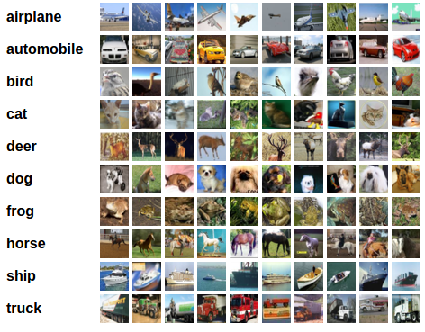
CIFAR 10
Train an Image Classifier
We will do the following steps in order:
- Load and normalizing the CIFAR10 training and test datasets using
torchvision - Define a Convolutional Neural Network
- Define a loss function
- Train the network on the training data
- Test the network on the test data
Load and normalize CIFAR10
import torch
import torchvision
import torchvision.transforms as transforms
The output of torchvision datasets are PILImage images of range [0, 1]. We transform them to Tensors of normalized range [-1, 1].
transform = transforms.Compose(
    [transforms.ToTensor(),
     transforms.Normalize((0.5, 0.5, 0.5), (0.5, 0.5, 0.5))]
)

# training set
trainset = torchvision.datasets.CIFAR10(root='./data', train=True,
                                        download=True, transform=transform)
trainloader = torch.utils.data.DataLoader(trainset, batch_size=4,
                                          shuffle=True, num_workers=2)

# test set
testset = torchvision.datasets.CIFAR10(root='./data', train=False,
                                       download=True, transform=transform)
testloader = torch.utils.data.DataLoader(testset, batch_size=4,
                                         shuffle=False, num_workers=2)

classes = ('plane', 'car', 'bird', 'cat',
           'deer', 'dog', 'frog', 'horse', 'ship', 'truck')
Define a CNN
import torch.nn as nn
import torch.nn.functional as F

class Net(nn.module):

    def __init__(self):
        super(Net, self).__init__()
        self.conv1 = nn.Conv2d(3, 6, 5)
        self.pool = nn.MaxPool2d(2, 2)
        self.conv2 = nn.Conv2d(6, 16, 5)
        self.fc1 = nn.Linear(16 * 5 * 5, 120)
        self.fc2 = nn.Linear(120, 84)
        self.fc3 = nn.Linear(84, 10)

    def forward(self, x):

        x = F.relu(self.conv1(x))
        x = self.pool(x)

        x = F.relu(self.conv2(x))
        x = self.pool(x)

        # flatten
        x = x.view(-1, 16 * 5 * 5)

        x = F.relu(self.fc1(x))
        x = F.relu(self.fc2(x))
        x = self.fc3(x)

        return x
net = Net()
print(net)
Net(
  (conv1): Conv2d(3, 6, kernel_size=(5, 5), stride=(1, 1))
  (pool): MaxPool2d(kernel_size=2, stride=2, padding=0, dilation=1, ceil_mode=False)
  (conv2): Conv2d(6, 16, kernel_size=(5, 5), stride=(1, 1))
  (fc1): Linear(in_features=400, out_features=120, bias=True)
  (fc2): Linear(in_features=120, out_features=84, bias=True)
  (fc3): Linear(in_features=84, out_features=10, bias=True)
)
Define loss function and optimizer
Here we will use a classification Cross-Entropy loss and SGD with momentum.
import torch.optim as optim

criterion = nn.CrossEntropyLoss()
optimizer = optim.SGD(net.parameters(), lr=0.001, momentum=0.9)
Train the network
- Loop over the training set multiple times. Each time
- Loop over our data iterator
- Zero the parameter gradients
- Forward pass: feed inputs to the network
- Compute loss
- Backpropagation
- Update parameters
- Loop over our data iterator
for epoch in range(2): # loop over the dataset multiple times
    running_loss = 0.0
    for i, data in enumerate(trainloader, 0):
        # get the inputs
        # data is a list of [inputs, labels]
        inputs, labels = data

        # zero the parameter gradients
        optimizer.zero_grad()

        # forward
        outputs = net(inputs)
        # compute loss
        loss = criterion(outputs, labels)
        # backward
        loss.backward()
        # update parameters
        optimizer.step()

        # print statistics
        running_loss += loss.item()
        if i % 2000 == 1999: # print every 2000 mini-batches
            print('[%d, %5d] loss: %.3f' %
                  (epoch + 1, i + 1, running_loss / 2000))
            running_loss = 0.0

print("Finished training!")
[1,  2000] loss: 2.171
[1,  4000] loss: 1.871
[1,  6000] loss: 1.675
[1,  8000] loss: 1.578
[1, 10000] loss: 1.500
[1, 12000] loss: 1.472
[2,  2000] loss: 1.408
[2,  4000] loss: 1.373
[2,  6000] loss: 1.334
[2,  8000] loss: 1.306
[2, 10000] loss: 1.311
[2, 12000] loss: 1.249
Finished training!
Save trained model
PATH = './cifar_net.pth'
torch.save(net.state_dict(), PATH)
Test the network
We will check this by predicting the class label that the neural network outputs, and checking it against the ground-truth. If the prediction is correct, we add the sample to the list of correct predictions.
Firstly, let’s load back in our saved model.
net = Net()
net.load_state_dict(torch.load(PATH))
Now let’s look at how the network performs on the test dataset:
correct, total = 0, 0
with torch.no_grad():
    for data in testloader:
        images, labels = data
        outputs = net(images)
        _, predicted = torch.max(outputs.data, 1)
        total += labels.size(0)
        # If the prediction is correct,
        # we add the sample to the list of correct predictions.
        correct += (predicted == labels).sum().item()

print('Accuracy of the network on the 10000 test images: %d %%' % (
    100 * correct / total))
Accuracy of the network on the 10000 test images: 56 %
Seems like the network learnt something! 👏
Train on GPU
Define our device as the first visible cuda device if we have CUDA available
device = torch.device("cuda:0" if torch.cuda.is_available() else "cpu") print(device)cuda:0Transfer the neural network as well as the data onto the GPU
# recursively go over all modules and
# convert their parameters and buffers to CUDA tensors
net.to(device)

# also send inputs and targets at every step to the GPU
inputs, labels = data[0].to(device), data[1].to(device)