Performance Measurement

Main Issues of Time Measurement

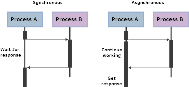
GPU Execution Mechanism: Asynchronous Execution

In multithreaded or multi-device programming, two blocks of code that are independent can be executed in parallel. This means that the second block may be executed before the first is finished. This process is referred to as asynchronous execution.

In the deep learning context, we often use this execution because the GPU operations are asynchronous by default.

• More specifically, when calling a function using a GPU, the operations are enqueued to the specific device, but not necessarily to other devices. This allows us to execute computations in parallel on the CPU or another GPU.

GPU Warm-up

A modern GPU device can exist in one of several different power states.

When the GPU is NOT being used for any purpose and persistence mode (i.e., which keeps the GPU on) is not enabled, the GPU will automatically reduce its power state to a very low level, sometimes even a complete shutdown. In lower power state, the GPU shuts down different pieces of hardware, including memory subsystems, internal subsystems, or even compute cores and caches.

In low power state, the invocation of any program that attempts to interact with the GPU will cause the driver to load and/or initialize the GPU. This driver load behavior is noteworthy! Applications that trigger GPU initialization can incur up to 3 seconds of latency, due to the scrubbing behavior of the error correcting code.

• For instance, if we measure time for a network that takes 10 milliseconds for one example, running over 1000 examples may result in most of our running time being wasted on initializing the GPU.

The Correct Way to Measure Inference Time

• Before we make any time measurements, we run some dummy examples through the network to do a ‘GPU warm-up.’ This will automatically initialize the GPU and prevent it from going into power-saving mode when we measure time.
• Next, we use torch.cuda.event to measure time on the GPU.
  • It is crucial here to use torch.cuda.synchronize(). This line of code performs synchronization between the host and device (i.e., GPU and CPU), so the time recording takes place only after the process running on the GPU is finished. This overcomes the issue of unsynchronized execution.

Code Snippet

import torch
import torchvision.models as models
import numpy as np
from tqdm import tqdm


device = torch.device("cuda")
model = models.resnet18(pretrained=True).to(device)
dummy_input = torch.randn([1, 3, 1024, 2048], dtype=torch.float).to(device)

# Init loggers
WARMUP_REPETITION = 100
MEASURE_REPETITION = 300
starter, ender = torch.cuda.Event(enable_timing=True), torch.cuda.Event(enable_timing=True)
infer_times = np.zeros((MEASURE_REPETITION,1))

# GPU warm-up
for _ in tqdm(range(WARMUP_REPETITION), desc="GPU warm-up", total=WARMUP_REPETITION):
    _ = model(dummy_input)

# Measure performance
with torch.no_grad():
    for rep in tqdm(range(MEASURE_REPETITION), desc="Measuring inference time", total=MEASURE_REPETITION):
        starter.record()
        _ = model(dummy_input)
        ender.record()

        # Wait for GPU sync
        torch.cuda.synchronize()

        curr_time = starter.elapsed_time(ender) # time unit is milliseconds
        curr_time = curr_time / 1000 # ms -> s
        infer_times[rep] = curr_time

mean_time = np.sum(infer_times) / MEASURE_REPETITION
std_time = np.std(infer_times)

print()
print(f"Mean: {mean_time:.3f} s, Std: {std_time:.3f} s")
print(f"FPS: {1 / mean_time:.3f}")

GPU warm-up: 100%|██████████| 100/100 [00:04<00:00, 24.66it/s]
Measuring inference time: 100%|██████████| 300/300 [00:13<00:00, 21.52it/s]
Mean: 44.390 s, Std: 0.890 s
FPS: 22.528

Common Mistakes when Measuring Time

When we measure the latency of a network, our goal is to measure only the feed-forward of the network (i.e. the inference), not more and not less.

Some common mistakes are listed below:

Transferring data between the host and the device

One of the most common mistakes involves the transfer of data between the CPU and GPU while taking time measurements. This is usually done unintentionally when a tensor is created on the CPU and inference is then performed on the GPU. This memory allocation takes a considerable amount of time, which subsequently enlarges the time for inference.

Not using GPU warm-up

The first run on the GPU prompts its initialization. GPU initialization can take up to 3 seconds, which makes a huge difference when the timing is in terms of milliseconds.

Using standard CPU timing

The most common mistake made is to measure time without synchronization.

Taking only one sample

A common mistake is to use ONLY one sample and refer to it as the run-time.

Like many processes in computer science, feed forward of the neural network has a (small) stochastic component. The variance of the run-time can be significant, especially when measuring a low latency network. To this end, it is essential to run the network over several examples and then average the results (300 examples can be a good number).

Measuring FPS

Once we have measured the inference time per image (in second), Frames Per Second (FPS) can be easily computed:

Measuring Throughput

The throughput of a neural network is defined as the maximal number of input instances the network can process in time a unit (e.g., a second). To achieve maximal throughput we would like to process in parallel as many instances as possible. The effective parallelism is obviously data-, model-, and device-dependent.

Thus, to correctly measure throughput we perform the following two steps:

1. We estimate the optimal batch size that allows for maximum parallelism

   • Rule of thumb: reach the memory limit of our GPU for the given data type
   • Using a for loop, we increase by one the batch size until Run Time error is achieved, this identifies the largest batch size the GPU can process, for our neural network model and the input data it processes.

2. Given this optimal batch size, we measure the number of instances the network can process in one second.

   • We process many batches (100 batches will be a sufficient number) and then use the following formula: $$ \frac{\text{\#batches} \times \text{batch size}}{\text{total time in seconds}} $$ This formula gives the number of examples our network can process in one second.

Code Snippet

import torch
import torchvision.models as models
import numpy as np
from tqdm import tqdm

# Assume that we have estimated the optimal batch size
device = torch.device("cuda")
model = models.resnet18(pretrained=True).to(device)
dummy_input = torch.randn([optimal_batch_size, 3, 1024, 2048], dtype=torch.float).to(device)

# Init loggers
MEASURE_REPETITION = 300
starter, ender = torch.cuda.Event(enable_timing=True), torch.cuda.Event(enable_timing=True)

total_time = 0

# Measure performance
with torch.no_grad():
    for rep in tqdm(range(MEASURE_REPETITION), desc="Measuring throughput", total=MEASURE_REPETITION):
        starter.record()
        _ = model(dummy_input)
        ender.record()

        # Wait for GPU sync
        torch.cuda.synchronize()

        curr_time = starter.elapsed_time(ender) / 1000
        total_time += curr_time

throughput = (MEASURE_REPETITION * optimal_batch_size) / total_time
print(f"Final Throughput: {throughput}")

Compute FLOPs

Firstly, we have to clearly distinguish between FLOPS and FLOPs

• FLOPS: floating point operations per second, is a measure of computer (hardware) performance, useful in fields of scientific computations that require floating-point calculations.
• FLOPs: floating point operations, is the amount of floating point operations, which is a metric for measurement of the complexity of a model or an algorithm.

To compute FLOPS, we can use fvcore. (More details see: Flop Counter for PyTorch Models)

Code example:

from fvcore.nn import FlopCountAnalysis

def get_FLOPs(model, dummy_input):
    flops = FlopCountAnalysis(model, dummy_input)
    return flops.total()

Reference

• The Correct Way to Measure Inference Time of Deep Neural Networks

• CNN 模型所需的计算力flops是什么？怎么计算？