Extended Kalman Filter
Motivation
Linear systems do not exist in reality. We have to deal with nonlinear discrete-time systems
$$ \begin{aligned} \underbrace{\mathbf{x}_{k}}_{\text{current state}}&=\mathbf{f}_{k-1}(\underbrace{\mathbf{x}_{k-1}}_{\text{previous state}}, \underbrace{\mathbf{u}_{k-1}}_{\text{inputs}}, \underbrace{\mathbf{w}_{k-1}}_{\text{process noise}}) \\\\ \underbrace{\mathbf{y}_{k}}_{\text{measurement}}&=\mathbf{h}_{k}(\mathbf{x}_{k}, \underbrace{\mathbf{v}_{k}}_{\text{measurement noise}}) \end{aligned} $$How can we adapt Kalman Filter to nonlinear discrete-time systems?
💡 Idea: Linearizing a Nonlinear System
Choose an operating point $a$ and approxiamte the nonlinear function by a tangent line at that point.
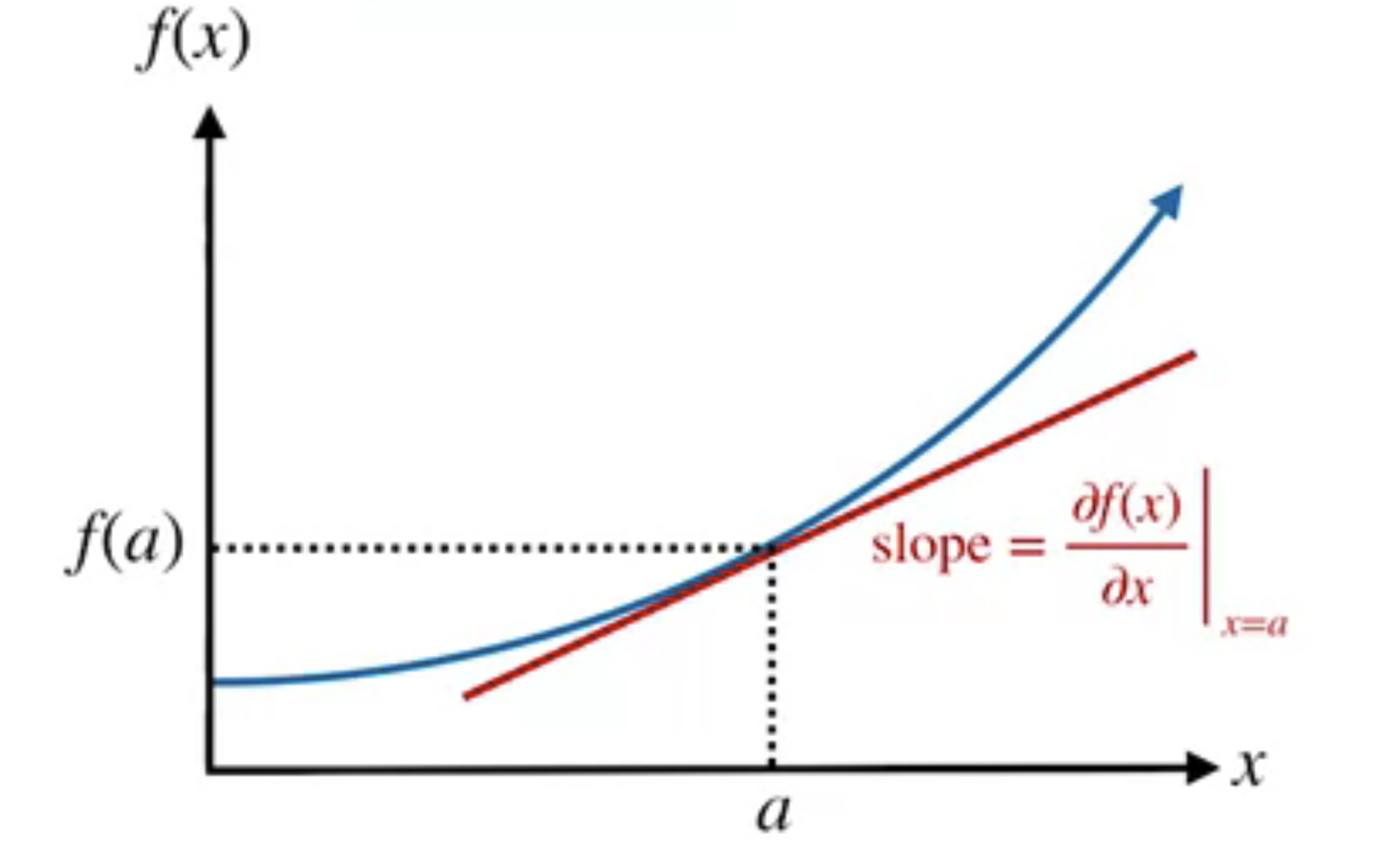
We compute this linear approximation using a first-order Taylor expansion
$$ f(x) \approx f(a)+\left.\frac{\partial f(x)}{\partial x}\right|_{x=a}(x-a) $$Extended Kalman Filter
For EKF, we choose the operationg point to be our most recent state estimate, our known input, and zero noise.
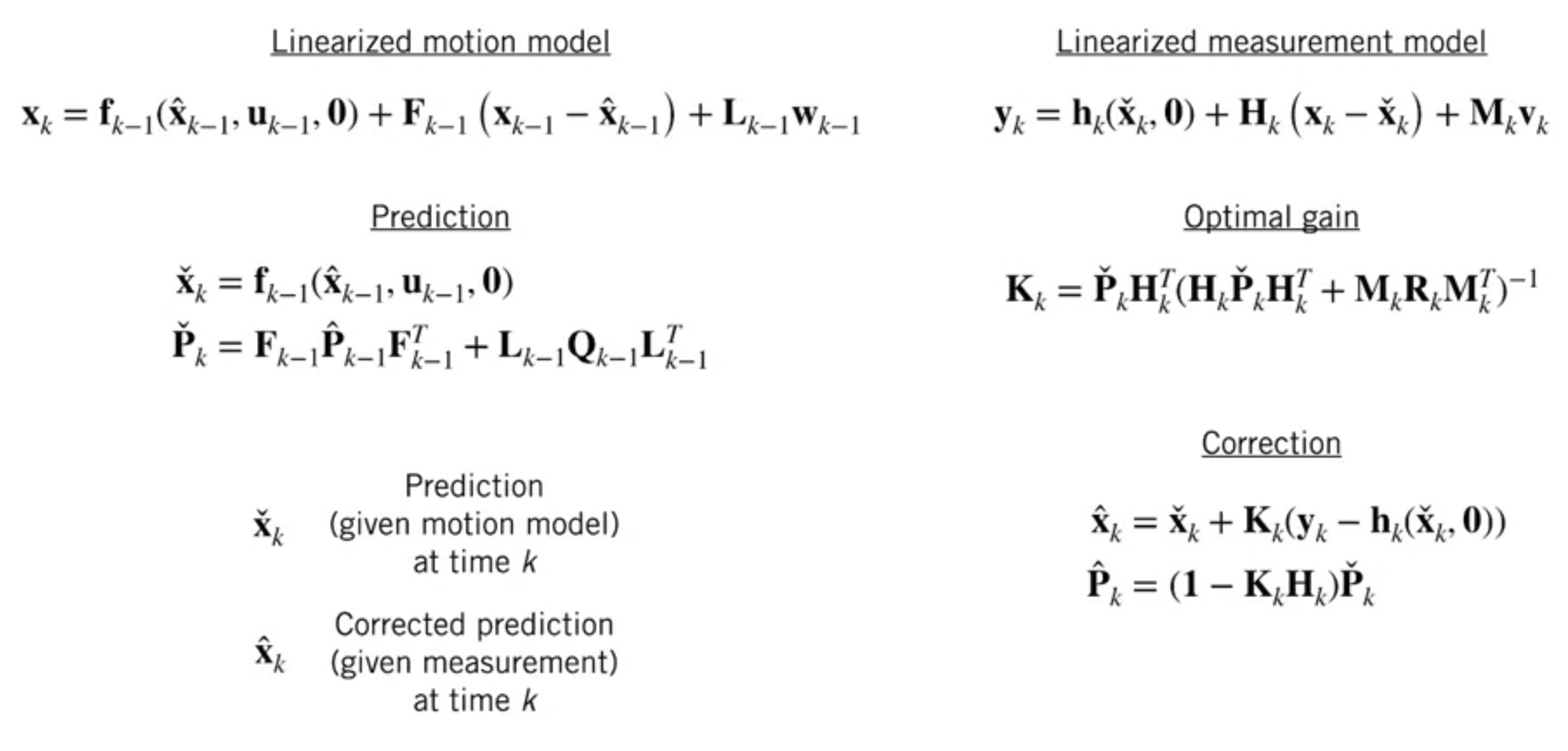
Linearized motion model
$$ \mathbf{x}_{k}=\mathbf{f}_{k-1}\left(\mathbf{x}_{k-1}, \mathbf{u}_{k-1}, \mathbf{w}_{k-1}\right) \approx \mathbf{f}_{k-1}\left(\hat{\mathbf{x}}_{k-1}, \mathbf{u}_{k-1}, \mathbf{0}\right) + \underbrace{\left.\frac{\partial \mathbf{f}_{k-1}}{\partial \mathbf{x}_{k-1}}\right|_{\hat{\mathbf{x}}_{k-1}, \mathbf{u}_{k-1}, \mathbf{0}}}_{\mathbf{F}_{k-1}}\left(\mathbf{x}_{k-1}-\hat{\mathbf{x}}_{k-1}\right)+\underbrace{\left.\frac{\partial \mathbf{f}_{k-1}}{\partial \mathbf{w}_{k-1}}\right|_{\hat{\mathbf{x}}_{k-1}, \mathbf{u}_{k-1}, \mathbf{0}}}_{\mathbf{L}_{k-1}} \mathbf{w}_{k-1} $$Linearized measurement model
$$ \mathbf{y}_{k}=\mathbf{h}_{k}\left(\mathbf{x}_{k}, \mathbf{v}_{k}\right) \approx \mathbf{h}_{k}\left(\check{\mathbf{x}}_{k}, \mathbf{0}\right)+\underbrace{\left.\frac{\partial \mathbf{h}_{k}}{\partial \mathbf{x}_{k}}\right|_{\check{\mathbf{x}}_{k}, \mathbf{0}}}_{\mathbf{H}_{k}}\left(\mathbf{x}_{k}-\check{\mathbf{x}}_{k}\right)+\underbrace{\left.\frac{\partial \mathbf{h}_{k}}{\partial \mathbf{v}_{k}}\right|_{\check{\mathbf{x}}_{k}, \mathbf{0}}}_{\mathbf{M}_{k}} \mathbf{v}_{k} $$
$\mathbf{F}_{k-1}, \mathbf{L}_{k-1}, \mathbf{H}_{k}, \mathbf{M}_{k}$ are Jacobian matrices.
Intuitively, the Jacobian matrix tells you how fast each output of the function is changing along each input dimension.
With our linearized models and Jacobians, we can now use the Kalman Filter equations.
Example
Similar to the self-driving car localisation example in Linear Kalman Fitler, but this time we use an onboard sensor, a camera, to measure the altitude of distant landmarks relative to the horizon.
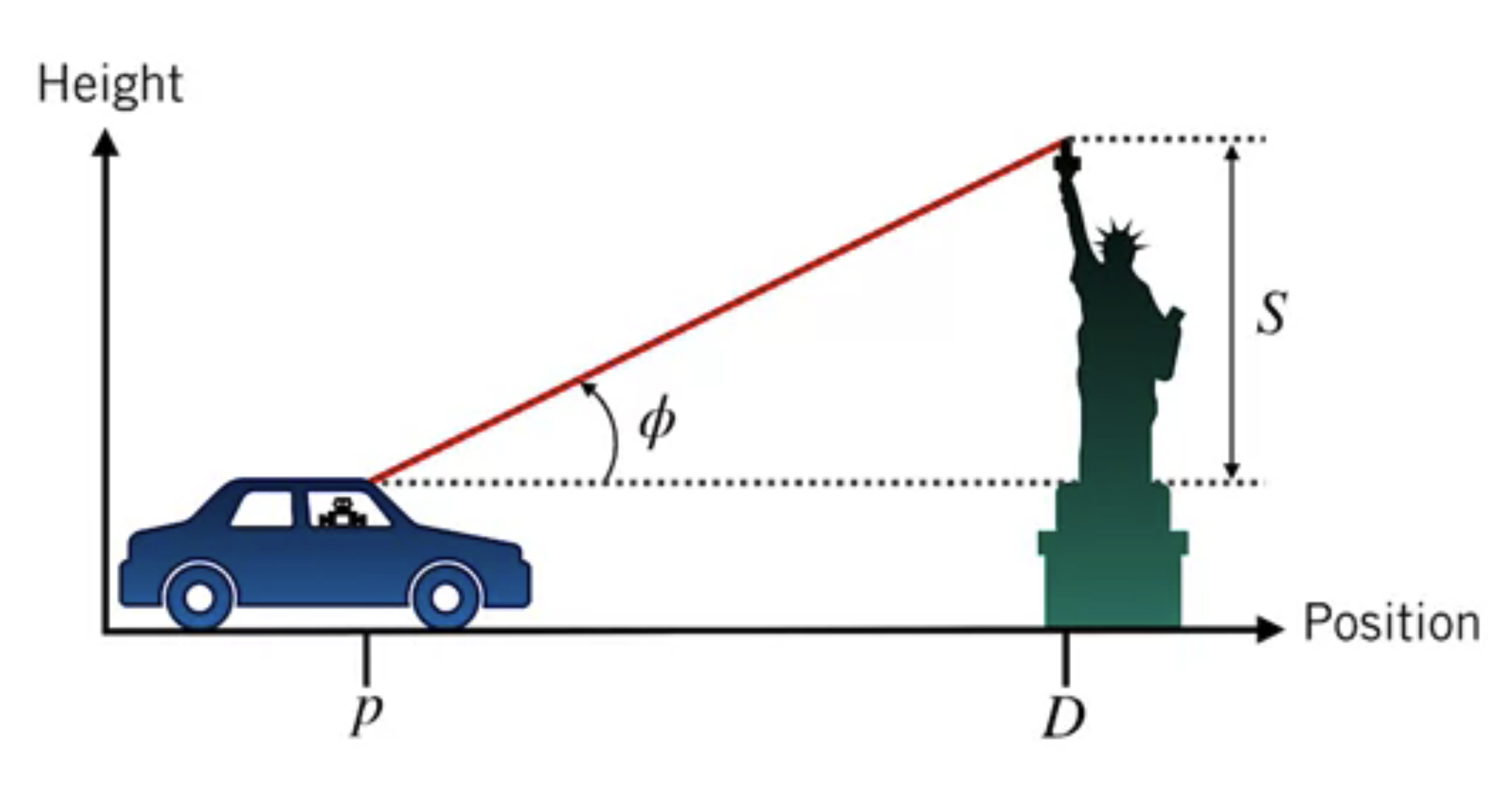
($S$ and $D$ are known in advance)
Sate:
$$ \mathbf{x}=\left[\begin{array}{l} p \\ \dot{p} \end{array}\right] $$Input:
$$ \mathbf{u}=\ddot{p} $$Motion/Process model
$$ \begin{aligned} \mathbf{x}_{k} &=\mathbf{f}\left(\mathbf{x}_{k-1}, \mathbf{u}_{k-1}, \mathbf{w}_{k-1}\right) \\\\ &=\left[\begin{array}{cc} 1 & \Delta t \\ 0 & 1 \end{array}\right] \mathbf{x}_{k-1}+\left[\begin{array}{c} 0 \\ \Delta t \end{array}\right] \mathbf{u}_{k-1}+\mathbf{w}_{k-1} \end{aligned} $$Landmark measurement model (nonlinear!)
$$ \begin{aligned} y_{k} &=\phi_{k}=h\left(p_{k}, v_{k}\right) \\\\ &=\tan ^{-1}\left(\frac{S}{D-p_{k}}\right)+v_{k} \end{aligned} $$Noise densities
$$ v_{k} \sim \mathcal{N}(0,0.01) \quad \mathbf{w}_{k} \sim \mathcal{N}\left(\mathbf{0},(0.1) \mathbf{1}_{2 \times 2}\right) $$The Jacobian matrices in this example are:
Motion model Jacobians
$$ \begin{array}{l} \mathbf{F}_{k-1}=\left.\frac{\partial \mathbf{f}}{\partial \mathbf{x}_{k-1}}\right|_{\hat{\mathbf{x}}_{k-1}, \mathbf{u}_{k-1}, \mathbf{0}}=\left[\begin{array}{cc} 1 & \Delta t \\ 0 & 1 \end{array}\right] \\\\ \mathbf{L}_{k-1}=\left.\frac{\partial \mathbf{f}}{\partial \mathbf{w}_{k-1}}\right|_{\hat{\mathbf{x}}_{k-1}, \mathbf{u}_{k-1}, \mathbf{0}}=\mathbf{1}_{2 \times 2} \end{array} $$Measurement model Jacobians
$$ \begin{array}{l} \mathbf{H}_{k}=\left.\frac{\partial h}{\partial \mathbf{x}_{k}}\right|_{\check{\mathbf{x}}_{k}, \mathbf{0}}=\left[\begin{array}{ll} \frac{S}{\left(D-\breve{p}_{k}\right)^{2}+S^{2}} & 0 \end{array}\right] \\\\ M_{k}=\left.\frac{\partial h}{\partial v_{k}}\right|_{\check{\mathbf{x}}_{k}, \mathbf{0}}=1 \end{array} $$
Given
$$ \begin{array}{l} \hat{\mathbf{x}}_{0} \sim \mathcal{N}\left(\left[\begin{array}{l} 0 \\ 5 \end{array}\right], \quad\left[\begin{array}{cc} 0.01 & 0 \\ 0 & 1 \end{array}\right]\right)\\ \Delta t=0.5 \mathrm{~s}\\ u_{0}=-2\left[\mathrm{~m} / \mathrm{s}^{2}\right] \quad y_{1}=\pi / 6[\mathrm{rad}]\\ S=20[m] \quad D=40[m] \end{array} $$What is the position estimate $\hat{p}_1$?
Prediction:
$$ \begin{array}{c} \check{\mathbf{x}}_{1}=\mathbf{f}_{0}\left(\hat{\mathbf{x}}_{0}, \mathbf{u}_{0}, \mathbf{0}\right) \\ {\left[\begin{array}{c} \check{p}_{1} \\ \dot{p}_{1} \end{array}\right]=\left[\begin{array}{cc} 1 & 0.5 \\ 0 & 1 \end{array}\right]\left[\begin{array}{l} 0 \\ 5 \end{array}\right]+\left[\begin{array}{c} 0 \\ 0.5 \end{array}\right](-2)=\left[\begin{array}{c} 2.5 \\ 4 \end{array}\right]} \\\\ \check{\mathbf{P}}_{1}=\mathbf{F}_{0} \hat{\mathbf{P}}_{0} \mathbf{F}_{0}^{T}+\mathbf{L}_{0} \mathbf{Q}_{0} \mathbf{L}_{0}^{T} \\ \check{\mathbf{P}}_{1}=\left[\begin{array}{cc} 1 & 0.5 \\ 0 & 1 \end{array}\right]\left[\begin{array}{cc} 0.01 & 0 \\ 0 & 1 \end{array}\right]\left[\begin{array}{cc} 1 & 0 \\ 0.5 & 1 \end{array}\right]+\left[\begin{array}{cc} 1 & 0 \\ 0 & 1 \end{array}\right]\left[\begin{array}{cc} 0.1 & 0 \\ 0 & 0.1 \end{array}\right]\left[\begin{array}{cc} 1 & 0 \\ 0 & 1 \end{array}\right]=\left[\begin{array}{cc} 0.36 & 0.5 \\ 0.5 & 1.1 \end{array}\right] \end{array} $$Correction:
$$ \begin{aligned} \mathbf{K}_{1} &=\check{\mathbf{P}}_{1} \mathbf{H}_{1}^{T}\left(\mathbf{H}_{1} \check{\mathbf{P}}_{1} \mathbf{H}_{1}^{T}+\mathbf{M}_{1} \mathbf{R}_{1} \mathbf{M}_{1}^{T}\right)^{-1} \\ &=\left[\begin{array}{cc} 0.36 & 0.5 \\ 0.5 & 1.1 \end{array}\right]\left[\begin{array}{c} 0.011 \\ 0 \end{array}\right]\left(\left[\begin{array}{ll} 0.011 & 0 \end{array}\right]\left[\begin{array}{cc} 0.36 & 0.5 \\ 0.5 & 1.1 \end{array}\right]\left[\begin{array}{c} 0.011 \\ 0 \end{array}\right]+1(0.01)(1)\right)^{-1} \\ &=\left[\begin{array}{c} 0.40 \\ 0.55 \end{array}\right] \end{aligned} $$ $$ \begin{aligned} \hat{\mathbf{x}}_{1} &=\check{\mathbf{x}}_{1}+\mathbf{K}_{1}\left(\mathbf{y}_{1}-\mathbf{h}_{1}\left(\check{\mathbf{x}}_{1}, \mathbf{0}\right)\right) \\ {\left[\begin{array}{c} \hat{p}_{1} \\ \hat{\dot{p}}_{1} \end{array}\right]}&={\left[\begin{array}{c} 2.5 \\ 4 \end{array}\right]+\left[\begin{array}{c} 0.40 \\ 0.55 \end{array}\right](0.52-0.49)=\left[\begin{array}{c} 2.51 \\ 4.02 \end{array}\right] } \end{aligned} $$ $$ \begin{aligned} \hat{\mathbf{P}}_{1} &=\left(\mathbf{1}-\mathbf{K}_{1} \mathbf{H}_{1}\right) \check{\mathbf{P}}_{1} \\ &=\left[\begin{array}{cc} 0.36 & 0.50 \\ 0.50 & 1.1 \end{array}\right] \end{aligned} $$Summary
The EKF uses linearization to adapt the Kalman Filter to nonlinear systems
Linearization works by computing a local linear apporximation to a nonlinear function using the first-order Taylor expansion on a chosen operating point (in this case, the last state estimate)