Kalman Filter
The Kalman filter is an efficient recursive filter estimating the internal-state of a linear dynamic system from a series of noisy measurements.
Applications of Kalman filter include
- Guidance
- Navigation
- Control of vehicles, aircraft, spacecraft, and ships positioned dynamically
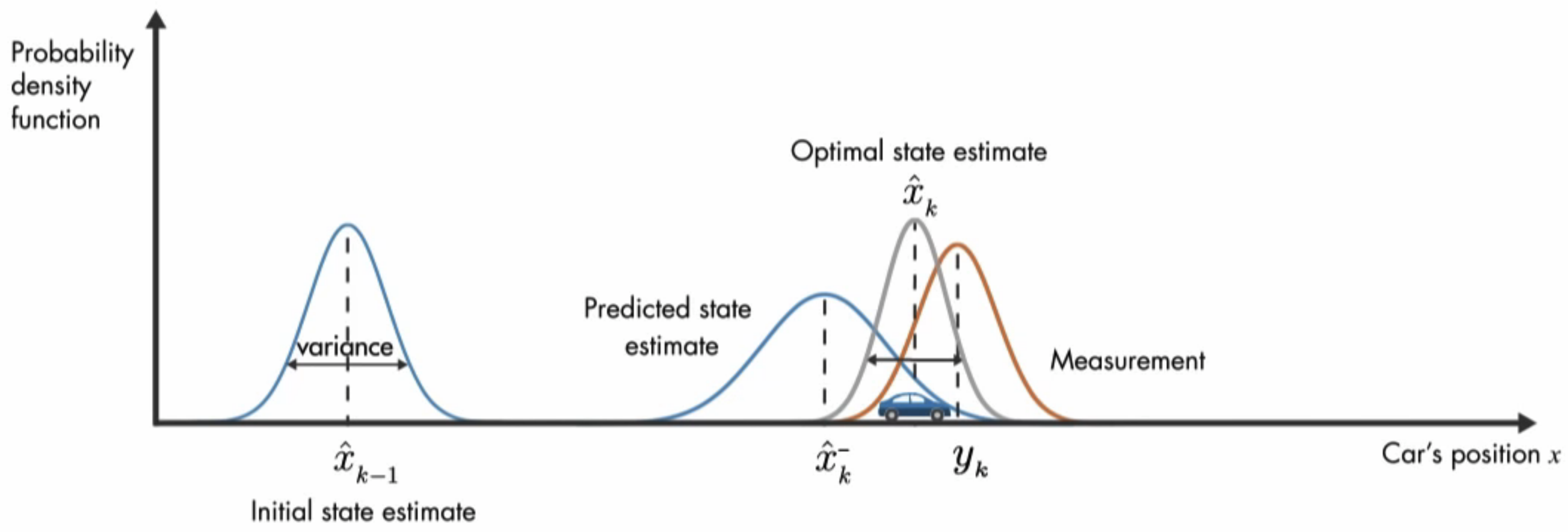
💡 The basic idea of Kalman filter is to achieve the optimal estimate of the (hidden) internal state by weightedly combining the state prediction and the measurement.
Kalman Filter Summary
Kalman filter in a picture:
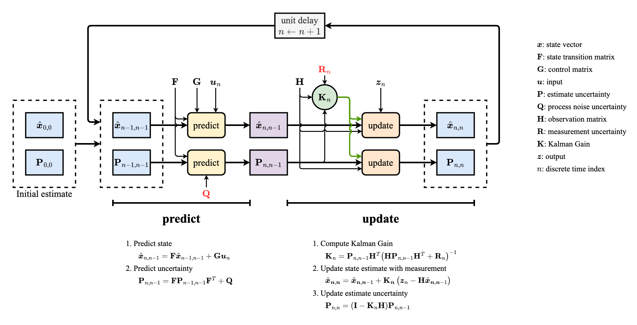
Summary of equations:
| Equation | Equation Name | Alternative Names | |
|---|---|---|---|
| Predict | $\hat{\boldsymbol{x}}_{n, n-1}=\mathbf{F} \hat{\boldsymbol{x}}_{n-1, n-1} + \mathbf{G} \boldsymbol{u}_{n}$ | State Extrapolation | Predictor Equation Transition Equation Prediction Equation Dynamic Model State Space Model |
| $\mathbf{P}_{n, n-1}=\mathbf{F} \mathbf{P}_{n-1, n-1} \mathbf{F}^{T}+\mathbf{Q}$ | Covariance Extrapolation | Predictor Covariance Equation | |
| Update | $\mathbf{K}_{n}=\mathbf{P}_{n, n-1} \mathbf{H}^{T}\left(\mathbf{H} \mathbf{P}_{n, n-1} \mathbf{H}^{T}+\mathbf{R}_{n}\right)^{-1}$ | Kalman Gain | Weight Equation |
| $\hat{\boldsymbol{x}}_{\boldsymbol{n}, \boldsymbol{n}}=\hat{\boldsymbol{x}}_{\boldsymbol{n}, \boldsymbol{n}-1}+\mathbf{K}_{\boldsymbol{n}}\left(\boldsymbol{z}_{n}-\mathbf{H} \hat{\boldsymbol{x}}_{\boldsymbol{n}, \boldsymbol{n}-1}\right)$ | State Update | Filtering Equation | |
| $\mathbf{P}_{n, n}=\left(\mathbf{I}-\mathbf{K}_{n} \mathbf{H}\right) \mathbf{P}_{n, n-1}$ | Covariance Update | Corrector Equation | |
| Auxilliary | $\boldsymbol{z}_{n} = \mathbf{H} \boldsymbol{x}_n + \boldsymbol{v}_n$ | Measurement Equation | |
| $\mathbf{R}_n = E\{\boldsymbol{v}_n \boldsymbol{v}_n^T\}$ | Measurement Uncertainty | Measurement Error | |
| $\mathbf{Q}_n = E\{\boldsymbol{w}_n \boldsymbol{w}_n^T\}$ | Process Noise Uncertainty | Process Noise Error | |
| $\mathbf{P}_{n, n}=E\left\{\boldsymbol{e}_{n} \boldsymbol{e}_{n}^{T}\right\}=E\left\{\left(\boldsymbol{x}_{n}-\hat{\boldsymbol{x}}_{n, n}\right)\left(\boldsymbol{x}_{n}-\hat{\boldsymbol{x}}_{n, n}\right)^{T}\right\}$ | Estimation Uncertainty | Estimation Error |
Summary of notations:
| Term | Name | Alternative Term |
|---|---|---|
| $\boldsymbol{x}$ | State vector | |
| $\boldsymbol{z}$ | Output vector | $\boldsymbol{y}$ |
| $\mathbf{F}$ | State transition matrix | $\mathbf{\Phi}$, $\mathbf{A}$ |
| $\boldsymbol{u}$ | Input variable | |
| $\mathbf{G}$ | Control matrix | $\boldsymbol{B}$ |
| $\mathbf{P}$ | Estimate uncertainty | $\boldsymbol{\Sigma}$ |
| $\mathbf{Q}$ | Process noise uncertainty | |
| $\mathbf{R}$ | Measurement uncertainty | |
| $\boldsymbol{w}$ | Process noise vector | |
| $\boldsymbol{v}$ | Measurement noise vector | |
| $\mathbf{H}$ | Observation matrix | $\mathbf{C}$ |
| $\mathbf{K}$ | Kalman Gain | |
| $n$ | Discrete time index | $k$ |
Multidimensional Kalman Filter in Detail
A Kalman filter works by a two-phase process, including 5 main equations:
- Predict phase: produces prediction of the current state, along with thier uncertainties
- Update phase: checks how good the predicted result fits to the current measurement and refines the state prediction using a weighted average given measurements if necessary.
State extrapolation equation
The Kalman filter assumes that the true state of a system at time step $n$ evolved from the prior state at time step $n-1$ is
$$ \boldsymbol{x}_n = \mathbf{F} \boldsymbol{x}_{n-1} +\mathbf{G} \boldsymbol{u}_{n} + \boldsymbol{w}_n $$$\boldsymbol{x}_{n}$ : state vector
$\boldsymbol{u}_{n}$ : control variable or input variable - a measurable (deterministic) input to the system
$\boldsymbol{w}_n$ : process noise or disturbance - an unmeasurable input that affects the state
$\mathbf{F}$ : state transition matrix - applies the effect of each system state parameter at time step $n-1$ on the system state at time step $n$
$\mathbf{G}$ : control matrix or input transition matrix (mapping control to state variables)
The state extrapolation equation
Predicts the next system state, based on the knowledge of the current state
Extrapolates the state vector from time step $n-1$ to $n$
Also called
- Predictor Equation
- Transition Equation
- Prediction Equation
- Dynamic Model
- State Space Model
The general form in a matrix notation
$$ \hat{\boldsymbol{x}}_{n, n-1}=\mathbf{F} \hat{\boldsymbol{x}}_{n-1, n-1}+\mathbf{G} \boldsymbol{u}_{n} $$$\hat{\boldsymbol{x}}_{n, n-1}$ : predicted system state vector at time step $n$
$\hat{\boldsymbol{x}}_{n-1, n-1}$ : estimated system state vector at time step $n-1$
$\hat{\boldsymbol{x}}_{n, m}$ represents the estimate of $\boldsymbol{x}$ at time step $n$ given observation/measurements up to and including at time $m \leq n$
Example
Covariance extrapolation equation
The covariance extrapolation equation extrapolates the uncertainty in our state prediction.
$$ \mathbf{P}_{n, n-1}=\mathbf{F} \mathbf{P}_{n-1, n-1} \mathbf{F}^{T}+\mathbf{Q} $$$\mathbf{P}_{n-1, n-1}$ : uncertainty (covariance matrix) of the estimate at time step $n-1$
$$ \begin{aligned} \mathbf{P}_{n-1, n-1} &= E\{\underbrace{(\boldsymbol{x}_{n-1, n-1} - \hat{\boldsymbol{x}}_{n-1, n-1})}_{=: \boldsymbol{e}_n} (\boldsymbol{x}_{n-1, n-1} - \hat{\boldsymbol{x}}_{n-1, n-1}) ^T\} \\ & = E\{\boldsymbol{e}_n \boldsymbol{e}_n^T\} \end{aligned} $$$\mathbf{P}_{n, n-1}$ : uncertainty (covariance matrix) of the prediction at time step $n$
$\mathbf{F}$ : state transition matrix
$\mathbf{Q}$ : process noise matrix
$$ \mathbf{Q}_n = E\{\boldsymbol{w}_n \boldsymbol{w}_n^T\} $$- $\boldsymbol{w}_n$ : process noise vector
Derivation
At time step $n$, the Kalman filter assumes
$$ \boldsymbol{x}\_n = \mathbf{F} \boldsymbol{x}\_{n-1} +\mathbf{G} \boldsymbol{u}\_{n} + \boldsymbol{w}\_n $$The prediction of state is
$$ \hat{\boldsymbol{x}}\_{n, n-1}=\mathbf{F} \hat{\boldsymbol{x}}\_{n-1, n-1}+\mathbf{G} \boldsymbol{u}\_{n} $$The difference between $\boldsymbol{x}\_n$ and $\hat{\boldsymbol{x}}\_{n, n-1}$ is
$$ \begin{aligned} \boldsymbol{x}\_{n}-\hat{\boldsymbol{x}}\_{n, n-1} &=\mathbf{F} \boldsymbol{x}\_{n-1}+\mathbf{G} \boldsymbol{u}\_{n}+\boldsymbol{w}\_{n}-\left(\mathbf{F} \hat{\boldsymbol{x}}\_{n-1, n-1}+\mathbf{G} \boldsymbol{u}\_{n}\right) \\\\ &=\mathbf{F}\left(\boldsymbol{x}\_{n-1}-\hat{\boldsymbol{x}}\_{n-1, n-1}\right)+\boldsymbol{w}\_{n} \end{aligned} $$The variance associate with the prediction $\hat{\boldsymbol{x}}\_{n, n-1}$ of an unknow true state $\boldsymbol{x}\_n$ is

Noting that the state estimation errors and process noise are uncorrelated:
$$ E\left\\{\left(\boldsymbol{x}\_{n-1}-\hat{\boldsymbol{x}}\_{n-1, n-1}\right) \boldsymbol{w}\_{n}^{T}\right\\} = E\left\\{\boldsymbol{w}\_{n}\left(\boldsymbol{x}\_{n-1}-\hat{\boldsymbol{x}}\_{n-1, n-1}\right)^{T}\right\\} = 0 $$Therefore
$$ \begin{aligned} \mathbf{P}\_{n, n-1} &=\underbrace{E\left\\{\left(\boldsymbol{x}\_{n-1}-\hat{\boldsymbol{x}}\_{n-1, n-1}\right)\left(\boldsymbol{x}\_{n-1}-\hat{\boldsymbol{x}}\_{n-1, n-1}\right)^{T}\right\\}}\_{=\mathbf{P}\_{n-1, n-1}} \mathbf{F}^{T}+\underbrace{E\left\\{w\_{n} w\_{n}^{T}\right\\}}\_{=\mathbf{Q}} \\\\ &=\mathbf{F} \mathbf{P}\_{n-1, n-1}\mathbf{F}^T+\mathbf{Q} \end{aligned} $$Kalman Gain equation
The Kalman Gain is calculated so that it minimizes the covariance of the a posteriori state estimate.
$$ \mathbf{K}_{n}=\mathbf{P}_{n, n-1} \mathbf{H}^{T}\left(\mathbf{H} \mathbf{P}_{n, n-1} \mathbf{H}^{T}+\mathbf{R}_{n}\right)^{-1} $$- $\mathbf{P}_{n, n-1}$ : uncertainty (covariance) matrix of the current state prediction
- $\mathbf{H}$ : observation matrix
- $\mathbf{R}_{n}$ : measurement Uncertainty (measurement noise covariance matrix)
Derivation
Rearrange the covariance update equation
$$ \begin{array}{l} \mathbf{P}\_{n, n}=\left(\mathbf{I}-\mathbf{K}\_{n} \mathbf{H}\right) \mathbf{P}\_{n, n-1}{\color{DodgerBlue} \left(\mathbf{I}-\mathbf{K}\_{n} \mathbf{H}\right)^{T}}+\mathbf{K}\_{n} \mathbf{R}\_{n} \mathbf{K}\_{n}^{T} \\\\\\\\ \mathbf{P}\_{n, n}=\left(\mathbf{I}-\mathbf{K}\_{n} \mathbf{H}\right) \mathbf{P}\_{n, n-1}{\color{DodgerBlue}\left(\mathbf{I}-\left(\mathbf{K}\_{n} \mathbf{H}\right)^{T}\right)}+\mathbf{K}\_{n} \mathbf{R}\_{n} \mathbf{K}\_{n}^{T} \qquad | \text{ } \mathbf{I} = \mathbf{I}^T \\\\\\\\ \mathbf{P}\_{n, n}={\color{ForestGreen}\left(\mathbf{I}-\mathbf{K}\_{n} \mathbf{H}\right) \mathbf{P}\_{n, n-1}}{\color{DodgerBlue}\left(\mathbf{I}-\mathbf{H}^{T} \mathbf{K}\_{n}^{T}\right)}+\mathbf{K}\_{n} \mathbf{R}\_{n} \mathbf{K}\_{n}^{T} \qquad | \text{ } (\mathbf{AB})^T = \mathbf{B}^T \mathbf{A}^T\\\\\\\\ \mathbf{P}\_{n, n}={\color{ForestGreen}\left(\mathbf{P}\_{n, n-1}-\mathbf{K}\_{n} \mathbf{H} \mathbf{P}\_{n, n-1}\right)}\left(\mathbf{I}-\mathbf{H}^{T} \mathbf{K}\_{n}^{T}\right)+\mathbf{K}\_{n} \mathbf{R}\_{n} \mathbf{K}\_{n}^{T} \\\\\\\\ \mathbf{P}\_{n, n}=\mathbf{P}\_{n, n-1}-\mathbf{P}\_{n, n-1} \mathbf{H}^{T} \mathbf{K}\_{n}^{T}-\mathbf{K}\_{n} \mathbf{H} \mathbf{P}\_{n, n-1} \\\\ +{\color{MediumOrchid}\mathbf{K}\_{n} \mathbf{H} \mathbf{P}\_{n, n-1} \mathbf{H}^{T} \mathbf{K}\_{n}^{T}+\mathbf{K}\_{n} \mathbf{R}\_{n} \mathbf{K}\_{n}^{T}} \qquad | \text{ } \mathbf{AB}\mathbf{A}^T + \mathbf{AC}\mathbf{A}^T = \mathbf{A}(\mathbf{B} + \mathbf{C})\mathbf{A}^T \\\\\\\\ \mathbf{P}\_{n, n}=\mathbf{P}\_{n, n-1}-\mathbf{P}\_{n, n-1} \mathbf{H}^{T} \mathbf{K}\_{n}^{T}-\mathbf{K}\_{n} \mathbf{H} \mathbf{P}\_{n, n-1} \\\\ +{\color{MediumOrchid}\mathbf{K}\_{n}\left(\mathbf{H} \mathbf{P}\_{n, n-1} \mathbf{H}^{T}+\boldsymbol{\mathbf{R}}\_{n}\right) \mathbf{K}\_{n}^{T}} \end{array} $$As the Kalman Filter is an optimal filter, we will seek a Kalman Gain that minimizes the estimate variance.
In order to minimize the estimate variance, we need to minimize the main diagonal (from the upper left to the lower right) of the covariance matrix $\mathbf{P}\_{n, n}$ .
The sum of the main diagonal of the square matrix is the trace of the matrix. Thus, we need to minimize $tr(\mathbf{P}\_{n, n})$ . In order to find the conditions required to produce a minimum, we will differentiate $tr(\mathbf{P}\_{n, n})$ w.r.t. $\mathbf{K}\_n$ and set the result to zero.
$$ \begin{array}{l} tr\left(\mathbf{P}\_{\boldsymbol{n}, \boldsymbol{n}}\right)=tr\left(\mathbf{P}\_{\boldsymbol{n}, \boldsymbol{n}-1}\right)-{\color{DarkOrange}tr\left(\mathbf{P}\_{n, n-1} \mathbf{H}^{T} \mathbf{K}\_{n}^{T}\right)}\\\\ {\color{DarkOrange} -tr\left(\mathbf{K}\_{n} \mathbf{H} \mathbf{P}\_{n, n-1}\right)} + tr\left(\mathbf{K}\_{\boldsymbol{n}}\left(\mathbf{H} \mathbf{P}\_{\boldsymbol{n}, \boldsymbol{n}-\mathbf{1}} \mathbf{H}^{\boldsymbol{T}}+\mathbf{R}\_{\boldsymbol{n}}\right) \mathbf{K}\_{n}^{\boldsymbol{T}}\right) \qquad | \text{} tr(\mathbf{A}) = tr(\mathbf{A}^T)\\\\\\\\ tr\left(\mathbf{P}\_{n, n}\right)=tr\left(\mathbf{P}\_{n, n-1}\right)-{\color{DarkOrange}2 tr\left(\mathbf{K}\_{n} \mathbf{H} \mathbf{P}\_{n, n-1}\right)}\\\\ +tr\left(\mathbf{K}\_{n}\left(\mathbf{H} \mathbf{P}\_{n, n-1} \mathbf{H}^{\boldsymbol{T}}+\mathbf{R}\_{n}\right) \mathbf{K}\_{n}^{T}\right)\\\\\\\\ \frac{d}{d \mathbf{K}\_{n}}t r\left(\mathbf{P}\_{n, n}\right)={\color{DodgerBlue} \frac{d}{d \mathbf{K}\_{n}}t r\left(\mathbf{P}\_{n, n-1}\right)}-{\color{ForestGreen}\frac{d }{d \mathbf{K}\_{n}}2 t r\left(\mathbf{K}\_{n} \mathbf{H} \mathbf{P}\_{n, n-1}\right)} \\\\ +{\color{MediumOrchid}\frac{d tr(\mathbf{K}\_{n}(\mathbf{H}\mathbf{P}\_{n, n-1}\mathbf{H}^T + \mathbf{R}\_n)\mathbf{K}\_{n}^T)}{d\mathbf{K}\_{n}}} \overset{!}{=} 0 \quad \mid {\color{ForestGreen} \frac{d}{d \mathbf{A}}tr(\mathbf{A} \mathbf{B}) = \mathbf{B}^T},{\color{MediumOrchid} \frac{d}{d \mathbf{A}}tr(\mathbf{A} \mathbf{B} \mathbf{A}^T) = 2\mathbf{A} \mathbf{B}}\\\\\\\\ \frac{d\left(t r\left(\mathbf{P}\_{n, n}\right)\right)}{d \mathbf{K}\_{n}}={\color{DodgerBlue}0}-{\color{ForestGreen}2\left(\mathbf{H} \mathbf{P}\_{ n , n - 1 }\right)^{T}}\\\\ +{\color{MediumOrchid}2 \mathbf{K}\_{n}\left(\mathbf{H} \mathbf{P}\_{n, n-1} \mathbf{H}^{T}+\mathbf{R}\_{n}\right)}=0\\\\\\\\ {\color{ForestGreen}\left(\mathbf{H} \mathbf{P}\_{n, n-1}\right)^{T}}={\color{MediumOrchid}\mathbf{K}\_{n}\left(\mathbf{H} \mathbf{P}\_{n, n-1} \mathbf{H}^{T}+\mathbf{R}\_{n}\right)} \\\\\\\\ \mathbf{K}\_{n}=\left(\mathbf{H} \mathbf{P}\_{n, n-1}\right)^{T}\left(\mathbf{H} \mathbf{P}\_{n, n-1} \mathbf{H}^{T}+\mathbf{R}\_{n}\right)^{-1} \quad \mid (\mathbf{AB})^T = \mathbf{B}^T \mathbf{A}^T \\\\\\\\ \mathbf{K}\_{n}=\mathbf{P}\_{n, n-1}^{T} \mathbf{H}^{T}\left(\mathbf{H} \mathbf{P}\_{n, n-1} \mathbf{H}^{T}+\mathbf{R}\_{n}\right)^{-1} \quad | \text{ covariance matrix } \mathbf{P} \text{ symmetric } (\mathbf{P}^T = \mathbf{P})\\\\\\\\ \mathbf{K}\_{n}=\mathbf{P}\_{n, n-1} \mathbf{H}^{T}\left(\mathbf{H} \mathbf{P}\_{n, n-1} \mathbf{H}^{T}+\mathbf{R}\_{n}\right)^{-1} \end{array} $$Kalman Gain intuition
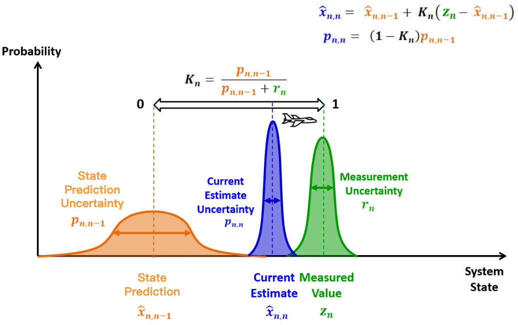
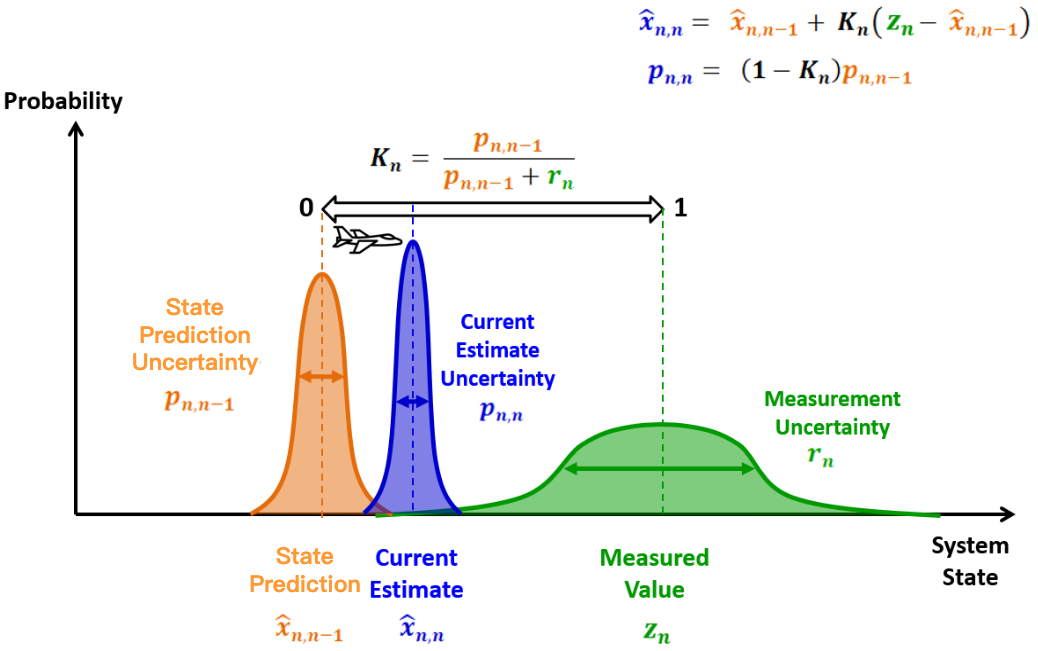
We show the intuition of Kalman Gain with a one-dimensional Kalman filter.
The one-dimensional Kalman Gain is
$$ \boldsymbol{K}_{\boldsymbol{n}}=\frac{p_{n, n-1}}{p_{n, n-1}+r_{n}} \in [0, 1] $$- $p_{n, n-1}$ : variance of the state prediction $\hat{x}_{n, n-1}$
- $r_n$ : variance of the measurement $z_n$
(Derivation see here)
Let’s rewrite the (one-dimensional) state update equation:
$$ \hat{x}_{n, n}=\hat{x}_{n, n-1}+K_{n}\left(z_{n}-\hat{x}_{n, n-1}\right)=\left(1-K_{n}\right) \hat{x}_{n, n-1}+K_{n} z_{n} $$The Kalman Gain $K_n$ is the weight that we give to the measurement. And $(1 - K_n)$ is the weight that we give to the state prediction.
High Kalman Gain
A low measurement uncertainty (small $r_n$) relative to the prediction uncertainty would result in a high Kalman Gain (close to 1). The new estimate would be close to the measurement.
💡 Intuition
small $r_n \rightarrow$ accurate measurements $\rightarrow$ place more weight on the measurements and thus conform to them
Low Kalman Gain
A high measurement uncertainty (large $r_n$) relative to the prediction uncertainty would result in a low Kalman Gain (close to 0). The new estimate would be close to the prediction.
💡 Intuition
large $r_n \rightarrow$ measurements are not accurate $\rightarrow$ place more weight on the prediction and trust them more
State update equation
The state update equation updates/refines/corrects the state prediction with measurements.
$$ \hat{\boldsymbol{x}}_{\boldsymbol{n}, \boldsymbol{n}}=\hat{\boldsymbol{x}}_{\boldsymbol{n}, \boldsymbol{n}-1}+\mathbf{K}_{\boldsymbol{n}}\underbrace{\left(\boldsymbol{z}_{n}-\mathbf{H} \hat{\boldsymbol{x}}_{\boldsymbol{n}, \boldsymbol{n}-1}\right)}_{\text{innovation}} $$$\hat{\boldsymbol{x}}_{n, n}$ : estimated system state vector at time step $n$
$\hat{\boldsymbol{x}}_{n, n-1}$ : predicted system state vector at time step $n$
$\mathbf{K}_{\boldsymbol{n}}$ : Kalman Gain
$\mathbf{H}$ : observation matrix
$\boldsymbol{z}_{n}$ : measurement at time step $n$
$$ \boldsymbol{z}_{n} = \mathbf{H} \boldsymbol{x}_n + \boldsymbol{v}_n $$$\boldsymbol{x}_n$ : true system state (hidden state)
$\boldsymbol{v}_n$ : measurement noise
$\rightarrow$ Measurement uncertainty $\mathbf{R}_n$ is given by
$$ \mathbf{R}_n = E\{\boldsymbol{v}_n \boldsymbol{v}_n^T\} $$
Covariance update equation
The covariance update equation updates the uncertainty of state estimate on the base of covariance prediction
$$ \mathbf{P}_{n, n}=\left(\mathbf{I}-\mathbf{K}_{n} \mathbf{H}\right) \mathbf{P}_{n, n-1}\left(\mathbf{I}-\mathbf{K}_{n} \mathbf{H}\right)^{T}+\mathbf{K}_{n} \mathbf{R}_{n} \mathbf{K}_{n}^{T} $$- $\mathbf{P}_{n, n}$ : estimate uncertainty (covariance) matrix of the current state
- $\mathbf{P}_{n, n-1}$ : uncertainty (covariance) matrix of the current state prediction
- $\mathbf{K}_{n}$ : Kalman Gain
- $\mathbf{H}$ : observation matrix
- $\mathbf{R}_{n}$ : measurement Uncertainty (measurement noise covariance matrix)
Derivation
According to state update equation:
$$ \begin{aligned} \hat{\boldsymbol{x}}\_{n, n} &= \hat{\boldsymbol{x}}\_{n, n-1}+\mathbf{K}\_{n}\left(\boldsymbol{z}\_{n}-\mathbf{H} \hat{\boldsymbol{x}}\_{n, n-1}\right) \\\\\\\\ &= \hat{\boldsymbol{x}}\_{n, n-1}+\mathbf{K}\_{n}\left(\mathbf{H} \boldsymbol{x}\_n + \boldsymbol{v}\_n-\mathbf{H} \hat{\boldsymbol{x}}\_{n, n-1}\right) \end{aligned} $$The estimation error between the true (hidden) state $\boldsymbol{x}\_n$ and estimate $\hat{\boldsymbol{x}}\_{n, n}$ is:
$$ \begin{aligned} \boldsymbol{e}\_n &= \boldsymbol{x}\_n - \hat{\boldsymbol{x}}\_{n, n} \\\\ &= \boldsymbol{x}\_n - \hat{\boldsymbol{x}}\_{n, n-1} - \mathbf{K}\_{n}\mathbf{H}\boldsymbol{x}\_n - \mathbf{K}\_{n}\boldsymbol{v}\_n + \mathbf{K}\_{n}\mathbf{H} \hat{\boldsymbol{x}}\_{n, n-1}\\\\ &= \boldsymbol{x}\_n - \hat{\boldsymbol{x}}\_{n, n-1} - \mathbf{K}\_{n}\mathbf{H}(\boldsymbol{x}\_n - \hat{\boldsymbol{x}}\_{n, n-1}) - \mathbf{K}\_{n}\boldsymbol{v}\_n \\\\ &= (\mathbf{I} - \mathbf{K}\_{n}\mathbf{H})(\boldsymbol{x}\_n - \hat{\boldsymbol{x}}\_{n, n-1}) - \mathbf{K}\_{n}\boldsymbol{v}\_n \end{aligned} $$Estimate Uncertainty
$$ \begin{array}{l} \boldsymbol{\mathbf{P}}\_{n, n}=E\left(\boldsymbol{e}\_{n} \boldsymbol{e}\_{n}^{T}\right)=E\left(\left(\boldsymbol{x}\_{n}-\hat{\boldsymbol{x}}\_{n, n}\right)\left(\boldsymbol{x}\_{n}-\hat{\boldsymbol{x}}\_{n, n}\right)^{T}\right) \qquad | \text{ Plug in } \boldsymbol{e}\_n\\\\\\\\ \boldsymbol{\mathbf{P}}\_{n, n}=E\left(\left(\left(\mathbf{I}-\mathbf{K}\_{n} \mathbf{H}\right)\left(\boldsymbol{x}\_{n}-\hat{x}\_{n, n-1}\right)-\mathbf{K}\_{n} v\_{n}\right) \right.\\\\ \left.\times\left(\left(\mathbf{I}-\mathbf{K}\_{n} \mathbf{H}\right)\left(\boldsymbol{x}\_{n}-\hat{x}\_{n, n-1}\right)-\mathbf{K}\_{n} v\_{n}\right)^{T}\right)\\\\\\\\ \mathbf{P}\_{n, n}=E\left(\left(\left(\mathbf{I}-\boldsymbol{\mathbf{K}}\_{n} \mathbf{H}\right)\left(\boldsymbol{x}\_{n}-\hat{\boldsymbol{x}}\_{n, n-1}\right)-\boldsymbol{\mathbf{K}}\_{n} v\_{n}\right) \right.\\\\ \left.\times\left(\left(\left(\mathbf{I}-\mathbf{K}\_{n} \mathbf{H}\right)\left(\boldsymbol{x}\_{n}-\hat{x}\_{n, n-1}\right)\right)^{T}-\left(\mathbf{K}\_{n} v\_{n}\right)^{T}\right)\right) \qquad | \text{ }(\mathbf{A} \mathbf{B})^{T}=\mathbf{B}^{T} \mathbf{A}^{T} \\\\\\\\ \mathbf{P}\_{n, n}=E\left(\left(\left(\mathbf{I}-\mathbf{K}\_{n} \mathbf{H}\right)\left(\boldsymbol{x}\_{n}-\hat{x}\_{n, n-1}\right)-\mathbf{K}\_{n} v\_{n}\right) \right. \\\\ \left.\times\left(\left(\boldsymbol{x}\_{n}-\hat{x}\_{n, n-1}\right)^{T}\left(\mathbf{I}-\mathbf{K}\_{n} \mathbf{H}\right)^{T}-\left(\mathbf{K}\_{n} v\_{n}\right)^{T}\right)\right)\\\\\\\\ \mathbf{P}\_{n, n}=E\left(\left(\mathbf{I}-\mathbf{K}\_{n} \mathbf{H}\right)\left(\boldsymbol{x}\_{n}-\hat{x}\_{n, n-1}\right)\left(\boldsymbol{x}\_{n}-\hat{\boldsymbol{x}}\_{n, n-1}\right)^{T}\left(\mathbf{I}-\mathbf{K}\_{n} \mathbf{H}\right)^{T}\right.\\\\ -\left(\mathbf{I}-\mathbf{K}\_{n} \mathbf{H}\right)\left(\boldsymbol{x}\_{n}-\hat{x}\_{n, n-1}\right)\left(\mathbf{K}\_{n} v\_{n}\right)^{T}\\\\ -\mathbf{K}\_{n} v\_{n}\left(\boldsymbol{x}\_{n}-\hat{x}\_{n, n-1}\right)^{T}\left(\mathbf{I}-\mathbf{K}\_{n} \mathbf{H}\right)^{T}\\\\ \left.+\mathbf{K}\_{n} v\_{n}\left(\mathbf{K}\_{n} v\_{n}\right)^{T}\right) \qquad | \text{ } E(X \pm Y)=E(X) \pm E(Y)\\\\\\\\ \mathbf{P}\_{n, n}=E\left(\left(\mathbf{I}-\mathbf{K}\_{n} \mathbf{H}\right)\left(\boldsymbol{x}\_{n}-\hat{x}\_{n, n-1}\right)\left(\boldsymbol{x}\_{n}-\hat{x}\_{n, n-1}\right)^{T}\left(\mathbf{I}-\mathbf{K}\_{n} \mathbf{H}\right)^{T}\right)\\\\ -\color{red}{E\left(\left(\mathbf{I}-\mathbf{K}\_{n} \mathbf{H}\right)\left(\boldsymbol{x}\_{n}-\hat{x}\_{n, n-1}\right)\left(\mathbf{K}\_{n} v\_{n}\right)^{T}\right)}\\\\ -\color{red}{E\left(\mathbf{K}\_{n} v\_{n}\left(\boldsymbol{x}\_{n}-\hat{x}\_{n, n-1}\right)^{T}\left(\mathbf{I}-\mathbf{K}\_{n} \mathbf{H}\right)^{T}\right)}\\\\ +E\left(\mathbf{K}\_{n} v\_{n}\left(\mathbf{K}\_{n} v\_{n}\right)^{T}\right) \end{array} $$$\boldsymbol{x}\_{n}-\hat{x}\_{n, n-1}$ is the error of the prior estimate in relation to the true value. It is uncorrelated with the current measurement noise $\boldsymbol{v}\_n$. The expectation value of the product of two independent variables is zero.
$$ \begin{aligned} \color{red}{E\left(\left(\mathbf{I}-\mathbf{K}\_{n} \mathbf{H}\right)\left(\boldsymbol{x}\_{n}-\hat{x}\_{n, n-1}\right)\left(\mathbf{K}\_{n} v\_{n}\right)^{T}\right)} = 0 \\\\ \color{red}{E\left(\mathbf{K}\_{n} v\_{n}\left(\boldsymbol{x}\_{n}-\hat{x}\_{n, n-1}\right)^{T}\left(\mathbf{I}-\mathbf{K}\_{n} \mathbf{H}\right)^{T}\right)} = 0 \end{aligned} $$Therefore
$$ \begin{array}{l} \mathbf{P}\_{n, n}=E\left(\left(\mathbf{I}-\mathbf{K}\_{n} \mathbf{H}\right)\left(\boldsymbol{x}\_{n}-\hat{x}\_{n, n-1}\right)\left(\boldsymbol{x}\_{n}-\hat{x}\_{n, n-1}\right)^{T}\left(\mathbf{I}-\mathbf{K}\_{n} \mathbf{H}\right)^{T}\right)\\\\ +{\color{DodgerBlue}{E\left(\mathbf{K}\_{n} v\_{n}\left(\mathbf{K}\_{n} v\_{n}\right)^{T}\right)}} \qquad | \text{ }(\mathbf{A} \mathbf{B})^{T}=\mathbf{B}^{T} \mathbf{A}^{T} \\\\\\\\ \mathbf{P}\_{n, n}=E\left(\left(\mathbf{I}-\mathbf{K}\_{n} \mathbf{H}\right)\left(\boldsymbol{x}\_{n}-\hat{x}\_{n, n-1}\right)\left(\boldsymbol{x}\_{n}-\hat{x}\_{n, n-1}\right)^{T}\left(\mathbf{I}-\mathbf{K}\_{n} \mathbf{H}\right)^{T}\right)\\\\ +{\color{DodgerBlue}{E\left(\mathbf{K}\_{n} v\_{n} v\_{n}^T \mathbf{K}\_{n}^T\right)}} \qquad | \text{ } E(a X)=a E(X) \\\\\\\\ \mathbf{P}\_{n, n} = \left(\mathbf{I}-\mathbf{K}\_{n} \mathbf{H}\right) {\color{ForestGreen}\underbrace{{E\left(\left(\boldsymbol{x}\_{n}-\hat{x}\_{n, n-1}\right)\left(\boldsymbol{x}\_{n}-\hat{x}\_{n, n-1}\right)^{T}\right)}}\_{=\mathbf{P}\_{n, n-1}}}\left(\mathbf{I}-\mathbf{K}\_{n} \mathbf{H}\right)^{T} +\mathbf{K}\_{n}{\color{DodgerBlue}{\underbrace{E\left( v\_{n} v\_{n}^T \right)}\_{=\mathbf{R}\_n}}} \mathbf{K}\_{n}^T \\\\\\\\ \mathbf{P}\_{n, n} = \left(\mathbf{I}-\mathbf{K}\_{n} \mathbf{H}\right) {\color{ForestGreen}\mathbf{P}\_{n, n-1}} \left(\mathbf{I}-\mathbf{K}\_{n} \mathbf{H}\right)^{T} +\mathbf{K}\_{n}{\color{DodgerBlue}\mathbf{R}\_n} \mathbf{K}\_{n}^T \end{array} $$In many textbook you can see a simplified form:
$$ \mathbf{P}_{n, n}=\left(\mathbf{I}-\mathbf{K}_{n} \mathbf{H}\right) \mathbf{P}_{n, n-1} $$This equation is elegant and easier to remember and in many cases it performs well.
However, even the smallest error in computing the Kalman Gain (due to round off) can lead to huge computation errors. The subtraction $\left(\mathbf{I}-\mathbf{K}_{n} \mathbf{H}\right)$ can lead to nonsymmetric matrices due to floating-point errors. Therefore this equation is numerically unstable!
Derivation of a simplified form of the Covariance Update Equation
Reference
👍 kalmnnfilter.net: clear and detaied tutorial for Kalman filter
- The $\alpha-\beta-\gamma$ filter: detailed introduction to Kalman filter
- One-dimensional Kalman filter with serveral elaborated numerical examples
- Multidimensional Kalman filter
👍 How a Kalman filter works, in pictures: Kalman filter explained intuitively in pictures
Understanding Kalman Filters: a series of video tutorials that intuitively explains Kalman Filter step by step
Kalman and Bayesian Filters in Python: Kalman filter (in Python) explained using Jupyter Notebook
Understanding the Basis of the Kalman Filter Via a Simple and Intuitive Derivation