Linear Kalman Filter

Intuition Example

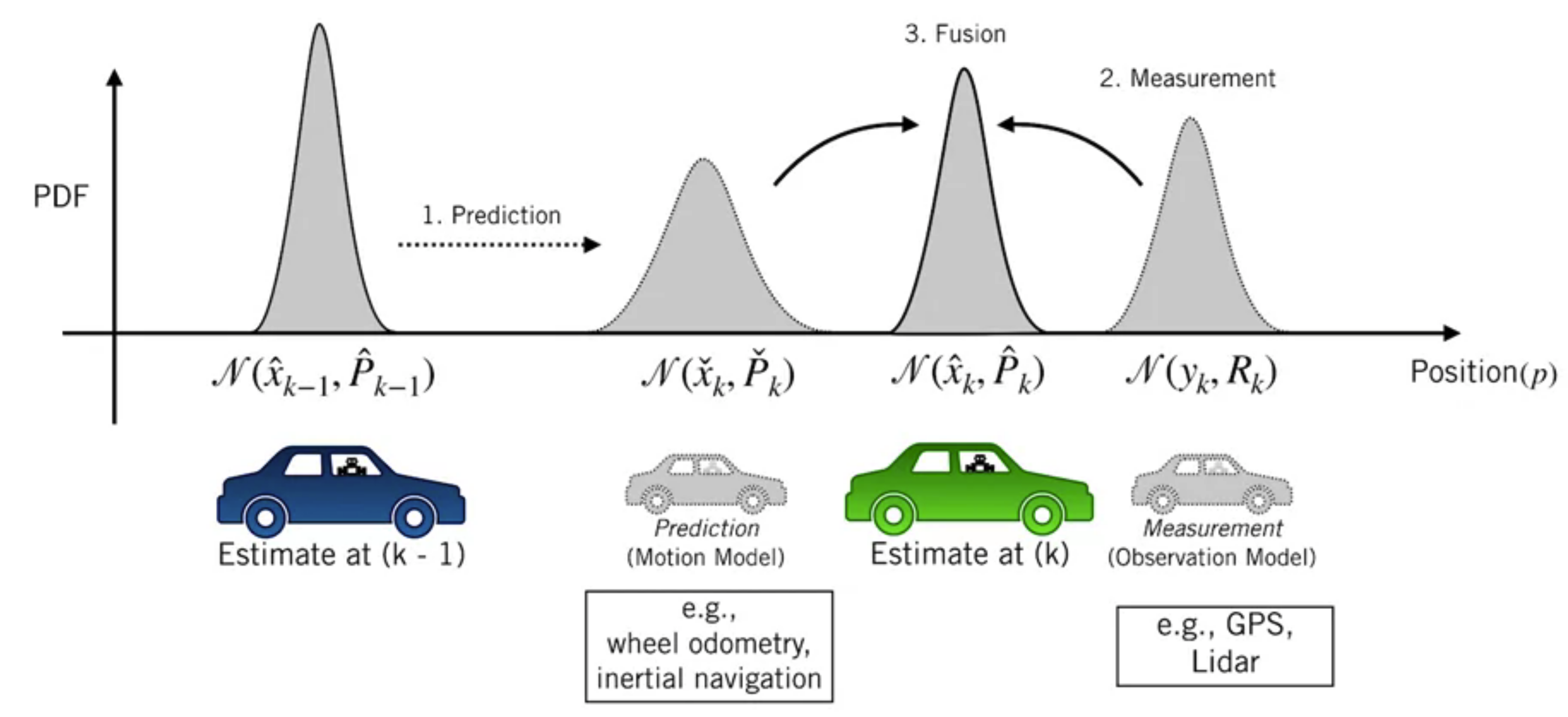
Estimation of the 1D position of the vehicle.

Starting from an initial probabilistic estimate at time $k-1$

Note: The initial estimate, the predicted state, and the final corrected state are all random variabless that we will specify their means and covariances.

1. Use a motion model to predict our new state
2. Use observation model (e.g. derived from GPS) to correct that prediction of vehicle position at time $k$

In this way, we can think of the Kalman filter as a technique to fuse information from different sensors to produce a final estimate of some unknown state, taking the uncertainty in motion and measurements into account.

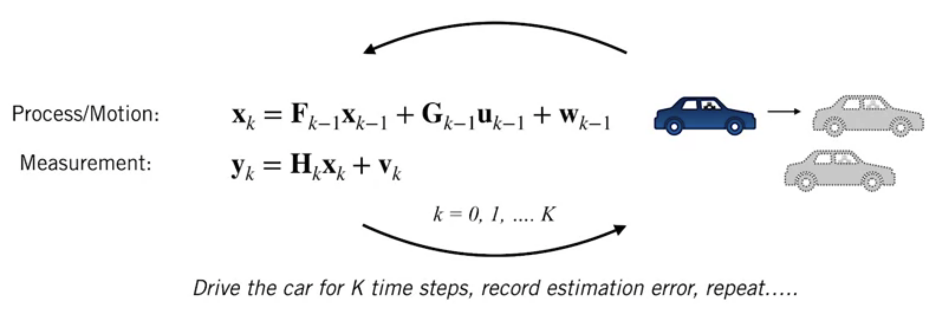
The Linear Dynamical System

Motion model:

$$ \mathbf{x}_{k}=\mathbf{F}_{k-1} \mathbf{x}_{k-1}+\mathbf{G}_{k-1} \mathbf{u}_{k-1}+\mathbf{w}_{k-1} $$

where

• $\mathbf{u}_k$: control input
• $\mathbf{w}_k$: process/motion noise. $\mathbf{w}_{k} \sim \mathcal{N}\left(\mathbf{0}, \mathbf{Q}_{k}\right)$

Measurement model

$$ \mathbf{y}_{k}=\mathbf{H}_{k} \mathbf{x}_{k}+\mathbf{v}_{k} $$

where

• $\mathbf{v}_{k}$: measurement noise. $\mathbf{v}_{k} \sim \mathcal{N}\left(\mathbf{0}, \mathbf{R}_{k}\right)$

Kalman Filter Steps

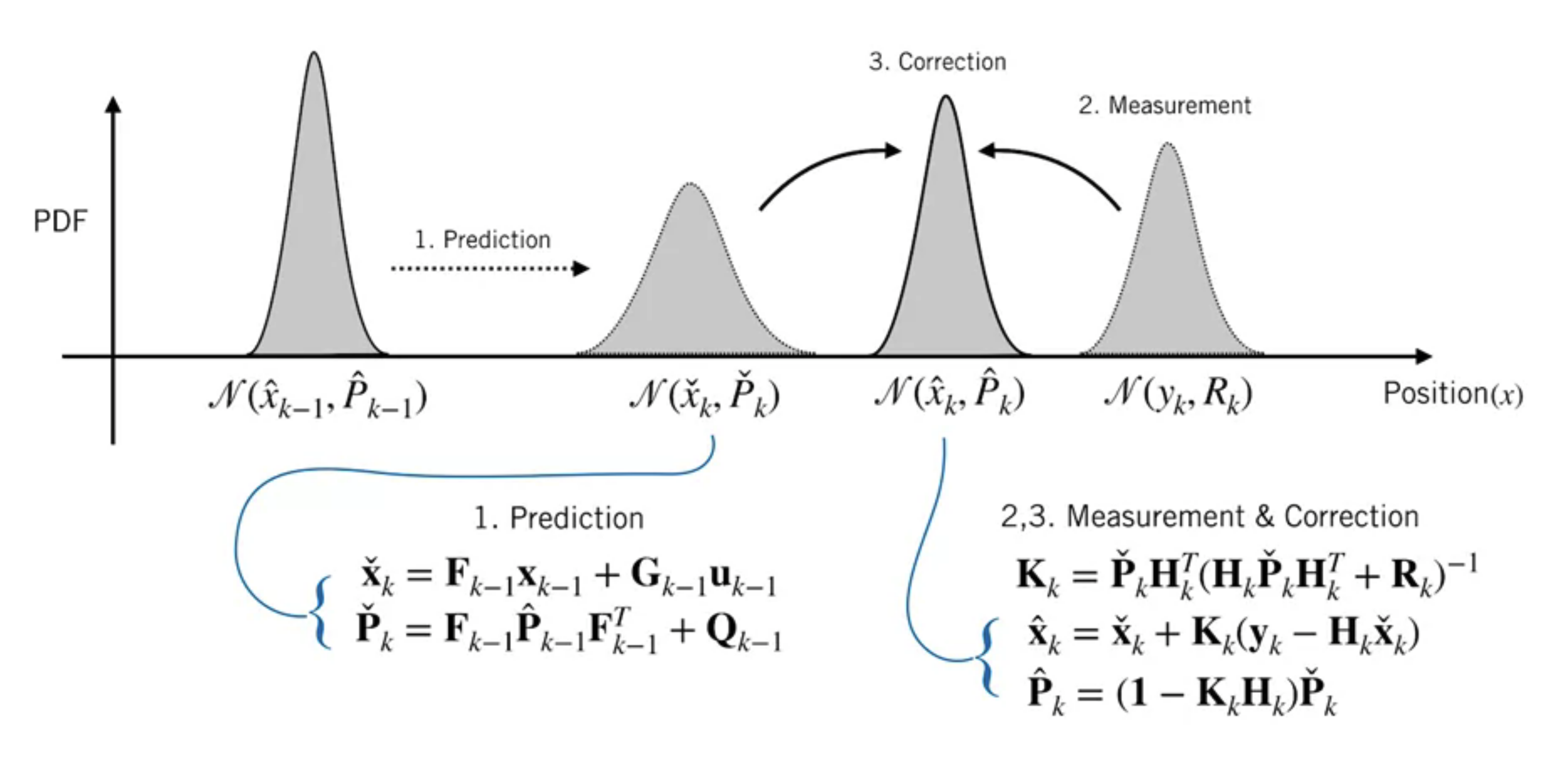
Prediction

We use the process model to predict how our state evolves since the last time step, and will propagate our uncertainty.

$$ \begin{array}{l} \check{\mathbf{x}}_{k}=\mathbf{F}_{k-1} \mathbf{x}_{k-1}+\mathbf{G}_{k-1} \mathbf{u}_{k-1} \\ \check{\mathbf{P}}_{k}=\mathbf{F}_{k-1} \hat{\mathbf{P}}_{k-1} \mathbf{F}_{k-1}^{T}+\mathbf{Q}_{k-1} \end{array} $$

Correction

We use measurement to correct that prediction

Notation:

• $\check{x}_k$: a prediction before the measurement is incorporated

• $\hat{x}_k$: corrected prediction at time step $k$

• Optimal Gain

  $$ \mathbf{K}_{k}=\check{\mathbf{P}}_{k} \mathbf{H}_{k}^{T}\left(\mathbf{H}_{k} \check{\mathbf{P}}_{k} \mathbf{H}_{k}^{T}+\mathbf{R}_{k}\right)^{-1} $$

• Correction

  $$ \begin{aligned} \hat{\mathbf{x}}_{k} &=\check{\mathbf{x}}_{k}+\mathbf{K}_{k}\underbrace{\left(\mathbf{y}_{k}-\mathbf{H}_{k} \check{\mathbf{x}}_{k}\right)}_{\text{innovation}} \\ \hat{\mathbf{P}}_{k}&=\left(\mathbf{I}-\mathbf{K}_{k} \mathbf{H}_{k}\right) \check{\mathbf{P}}_{k} \end{aligned} $$

Summary

Example

Consider a self-driving vehicle estimating its own position.

The state vector includes the position and its first derivative, velocity.

$$ \mathbf{x}=\left[\begin{array}{c} p \\ \frac{d p}{d t}=\dot{p} \end{array}\right] $$

Input is the scalar acceleration

$$ \mathbf{u}=a=\frac{d^{2} p}{d t^{2}} $$

THe linear dynamical system is

• Motion/Process model

  $$ \mathbf{x}_{k}=\left[\begin{array}{cc} 1 & \Delta t \\ 0 & 1 \end{array}\right] \mathbf{x}_{k-1}+\left[\begin{array}{c} 0 \\ \Delta t \end{array}\right] \mathbf{u}_{k-1}+\mathbf{w}_{k-1} $$

• Position observation

  $$ y_{k}=\left[\begin{array}{ll} 1 & 0 \end{array}\right] \mathbf{x}_{k}+v_{k} $$

• Nose densities

  $$ v_{k} \sim \mathcal{N}(0,0.05) \quad \mathbf{w}_{k} \sim \mathcal{N}\left(\mathbf{0},(0.1) \mathbf{1}_{2 \times 2}\right) $$

Given the data at time step $k=0$

$$ \begin{array}{l} \hat{\mathbf{x}}_{0} \sim \mathcal{N}\left(\left[\begin{array}{l} 0 \\ 5 \end{array}\right],\left[\begin{array}{cc} 0.01 & 0 \\ 0 & 1 \end{array}\right]\right) \\ \Delta t=0.5 \mathrm{~s} \\ u_{0}=-2\left[\mathrm{~m} / \mathrm{s}^{2}\right] \quad y_{1}=2.2[\mathrm{~m}] \end{array} $$

We want to estimate the state at time step $k=1$.

Prediction step

$$ \begin{aligned} \check{\mathbf{x}}_{k} &=\mathbf{F}_{k-1} \mathbf{x}_{k-1}+\mathbf{G}_{k-1} \mathbf{u}_{k-1} \\\\ {\left[\begin{array}{c} \check{p}_{1} \\ \check{p}_{1} \end{array}\right] } &=\left[\begin{array}{cc} 1 & 0.5 \\ 0 & 1 \end{array}\right]\left[\begin{array}{l} 0 \\ 5 \end{array}\right]+\left[\begin{array}{c} 0 \\ 0.5 \end{array}\right](-2)=\left[\begin{array}{c} 2.5 \\ 4 \end{array}\right] \end{aligned} $$ $$ \begin{aligned} \check{\mathbf{P}}_{k} &=\mathbf{F}_{k-1} \hat{\mathbf{P}}_{k-1} \mathbf{F}_{k-1}^{T}+\mathbf{Q}_{k-1} \\\\ \check{\mathbf{P}}_{1} &=\left[\begin{array}{cc} 1 & 0.5 \\ 0 & 1 \end{array}\right]\left[\begin{array}{cc} 0.01 & 0 \\ 0 & 1 \end{array}\right]\left[\begin{array}{cc} 1 & 0.5 \\ 0 & 1 \end{array}\right]^{T}+\left[\begin{array}{cc} 0.1 & 0 \\ 0 & 0.1 \end{array}\right]=\left[\begin{array}{cc} 0.36 & 0.5 \\ 0.5 & 1.1 \end{array}\right] \end{aligned} $$

Correction step

• Kalman Gain

  $$ \begin{aligned} \mathbf{K}_{1} &=\check{\mathbf{P}}_{1} \mathbf{H}_{1}^{T}\left(\mathbf{H}_{1} \check{\mathbf{P}}_{1} \mathbf{H}_{1}^{T}+\mathbf{R}_{1}\right)^{-1} \\ &\left.=\left[\begin{array}{cc} 0.36 & 0.5 \\ 0.5 & 1.1 \end{array}\right]\left[\begin{array}{l} 1 \\ 0 \end{array}\right]\left(\begin{array}{ll} 1 & 0 \end{array}\right]\left[\begin{array}{cc} 0.36 & 0.5 \\ 0.5 & 1.1 \end{array}\right]\left[\begin{array}{l} 1 \\ 0 \end{array}\right]+0.05\right)^{-1} \\ &=\left[\begin{array}{l} 0.88 \\ 1.22 \end{array}\right] \end{aligned} $$

• Correction of the state prediction

  $$ \begin{aligned} \hat{\mathbf{x}}_{1} &=\check{\mathbf{x}}_{1}+\mathbf{K}_{1}\left(\mathbf{y}_{1}-\mathbf{H}_{1} \check{\mathbf{x}}_{1}\right) \\\\ {\left[\begin{array}{c} \hat{p}_{1} \\ \hat{\dot{p}}_{1} \end{array}\right] } &=\left[\begin{array}{c} 2.5 \\ 4 \end{array}\right]+\left[\begin{array}{c} 0.88 \\ 1.22 \end{array}\right]\left(2.2-\left[\begin{array}{ll} 1 & 0 \end{array}\right]\left[\begin{array}{c} 2.5 \\ 4 \end{array}\right]\right)=\left[\begin{array}{l} 2.24 \\ 3.63 \end{array}\right] \end{aligned} $$

• Correction of covariance

  $$ \begin{aligned} \hat{\mathbf{P}}_{1} &=\left(\mathbf{1}-\mathbf{K}_{1} \mathbf{H}_{1}\right) \check{\mathbf{P}}_{1} \\\\ &=\left[\begin{array}{ll} 0.04 & 0.06 \\ 0.06 & 0.49 \end{array}\right] \end{aligned} $$

  Note that the final covariance (i.e. the covariance after correction) is smaller. That is, we are more certain about the car position after we incoporate the position measurement. This uncertainty reduction occurs because our measurement model is fairly accurate (the measurement noise variance is quite small).

Best Linear Unbiased Estimator (BLUE)

If we have white, uncorrelated zero-mean noise, the Kalman Fitler is the best (i.e., lowest variance) unbiased estimator that uses only a linear combination of measurements.

Bias

We repeat the above Kalman filter for $K$ times.

The bias is defined as the difference between true position and the mean of estimated position values.

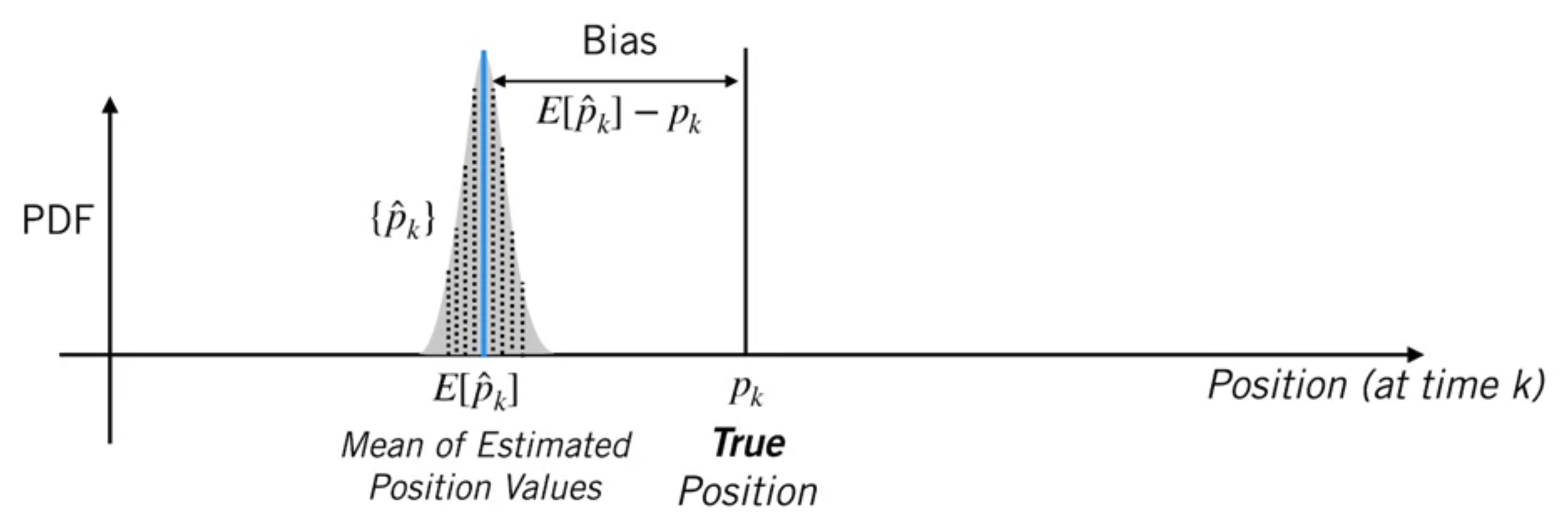
An estimator of filter is unbiased if it produces an “average” error of zero at a particular time step $k$, over many trials.

$$ E\left[\hat{e}_{k}\right]=E\left[\hat{p}_{k}-p_{k}\right]=E\left[\hat{p}_{k}\right]-p_{k}=0 \qquad \forall k \in \mathbb{N} $$

Bias in Kalman filter state estimation

Consider the error dynamics

• Predicted state error

  $$ \check{\mathbf{e}}_{k}=\check{\mathbf{x}}_{k}-\mathbf{x}_{k} $$

• Corrected state error

  $$ \hat{\mathbf{e}}_{k}=\hat{\mathbf{x}}_{k}-\mathbf{x}_{k} $$

Using the Kalman Fitler equations, we can derive

$$ \begin{array}{l} \check{\mathbf{e}}_{k}=\mathbf{F}_{k-1} \check{\mathbf{e}}_{k-1}-\mathbf{w}_{k} \\ \hat{\mathbf{e}}_{k}=\left(\mathbf{1}-\mathbf{K}_{k} \mathbf{H}_{k}\right) \check{\mathbf{e}}_{k}+\mathbf{K}_{k} \mathbf{v}_{k} \end{array} $$

So long as

• The initial state estimate is unbiased ($E\left[\hat{\mathbf{e}}_{0}\right]=\mathbf{0}$ )
• The noise is white, uncorrelated and zero mean ($E[\mathbf{v}]=\mathbf{0}, E[\mathbf{w}]=\mathbf{0}$ )

Then the state estiamte is unbiased

$$ \begin{aligned} E\left[\check{\mathbf{e}}_{k}\right] &=E\left[\mathbf{F}_{k-1} \check{\mathbf{e}}_{k-1}-\mathbf{w}_{k}\right] \\ &=\mathbf{F}_{k-1} E\left[\check{\mathbf{e}}_{k-1}\right]-E\left[\mathbf{w}_{k}\right] \\ &=\mathbf{0} \end{aligned} $$ $$ \begin{aligned} E\left[\hat{\mathbf{e}}_{k}\right] &=E\left[\left(\mathbf{1}-\mathbf{K}_{k} \mathbf{H}_{k}\right) \check{\mathbf{e}}_{k}+\mathbf{K}_{k} \mathbf{v}_{k}\right] \\ &=\left(\mathbf{1}-\mathbf{K}_{k} \mathbf{H}_{k}\right) E\left[\check{\mathbf{e}}_{k}\right]+\mathbf{K}_{k} E\left[\mathbf{v}_{k}\right] \\ &=\mathbf{0} \end{aligned} $$

Consistency

A filter is consistent if for all $k$

$$ E\left[\hat{e}_{k}^{2}\right]=E\left[\left(\hat{p}_{k}-p_{k}\right)^{2}\right]=\hat{P}_{k} $$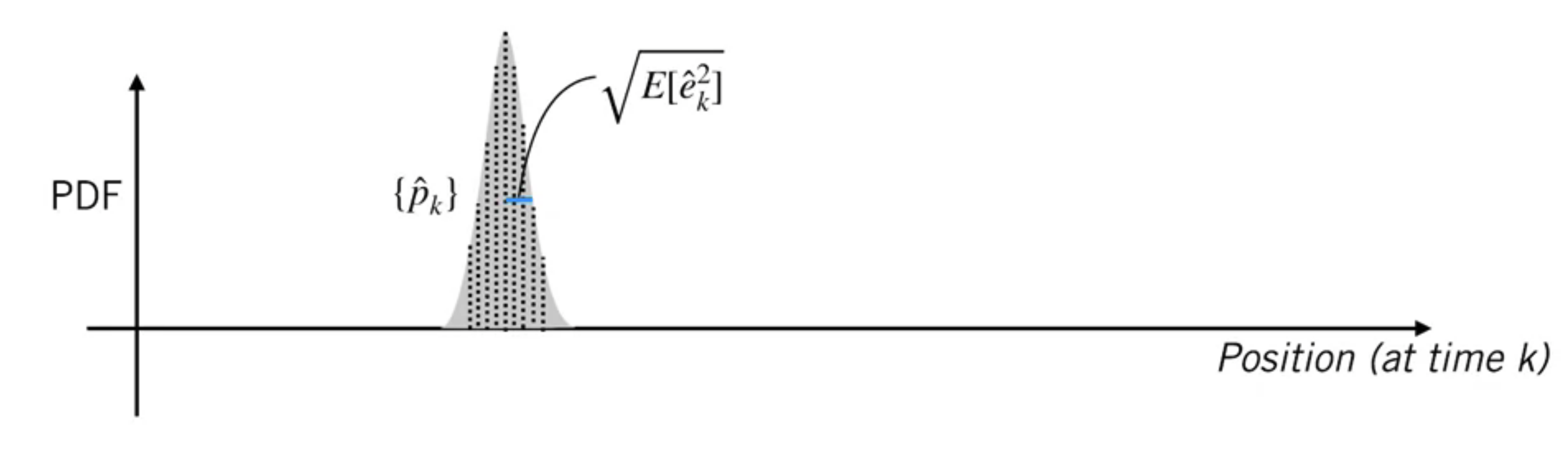

This means that the filter is neither overconfident nor underconfident in the estimate it has produced.

The Kalman Fitler is consistent in state estimate.

$$ E\left[\check{\mathbf{e}}_{k} \check{\mathbf{e}}_{k}^{T}\right]=\check{\mathbf{P}}_{k} \qquad E\left[\hat{\mathbf{e}}_{k} \hat{\mathbf{e}}_{k}^{T}\right]=\hat{\mathbf{P}}_{k} $$

so long as

• the initial state estimate is consistent ($E\left[\hat{\mathbf{e}}_{0} \hat{\mathbf{e}}_{0}^{T}\right]=\check{\mathbf{P}}_{0}$ )
• the noise is white and zero-mean ($E[\mathbf{v}]=\mathbf{0}, E[\mathbf{w}]=\mathbf{0}$ )

Reference

• The (Linear) Kalman Filter