Unscented Kalman Filter

Intuition

“It is easier to approximate a probability distribution than it is to approximate an arbitrary nonlinear function”

Idea

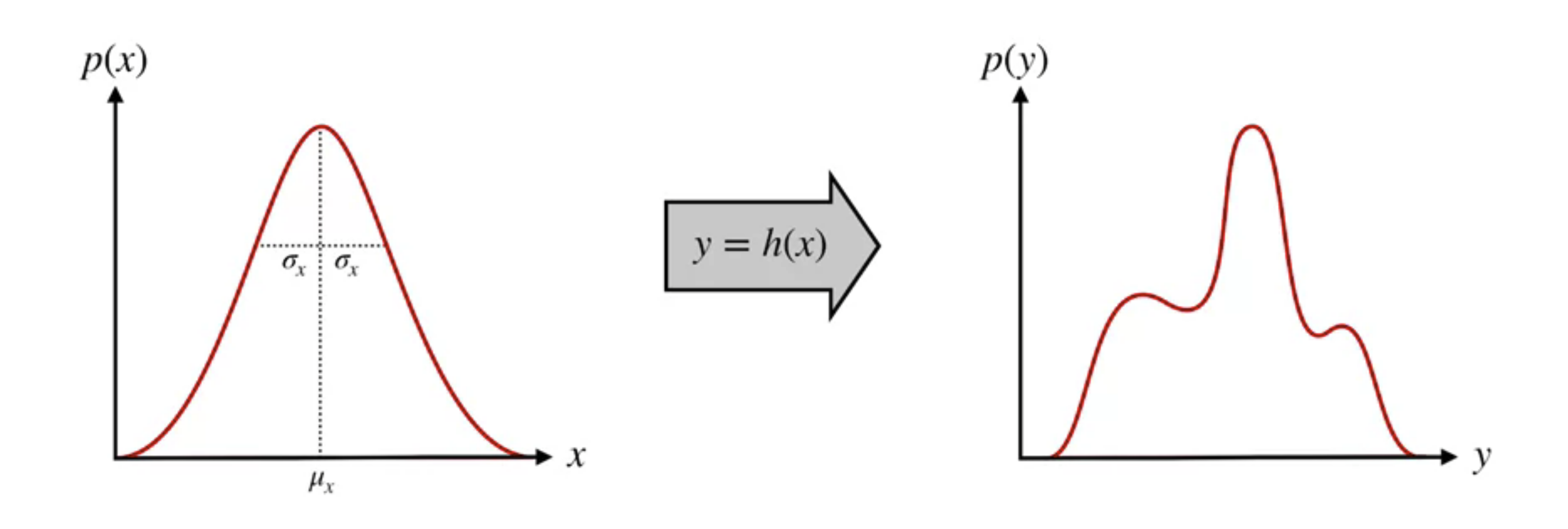
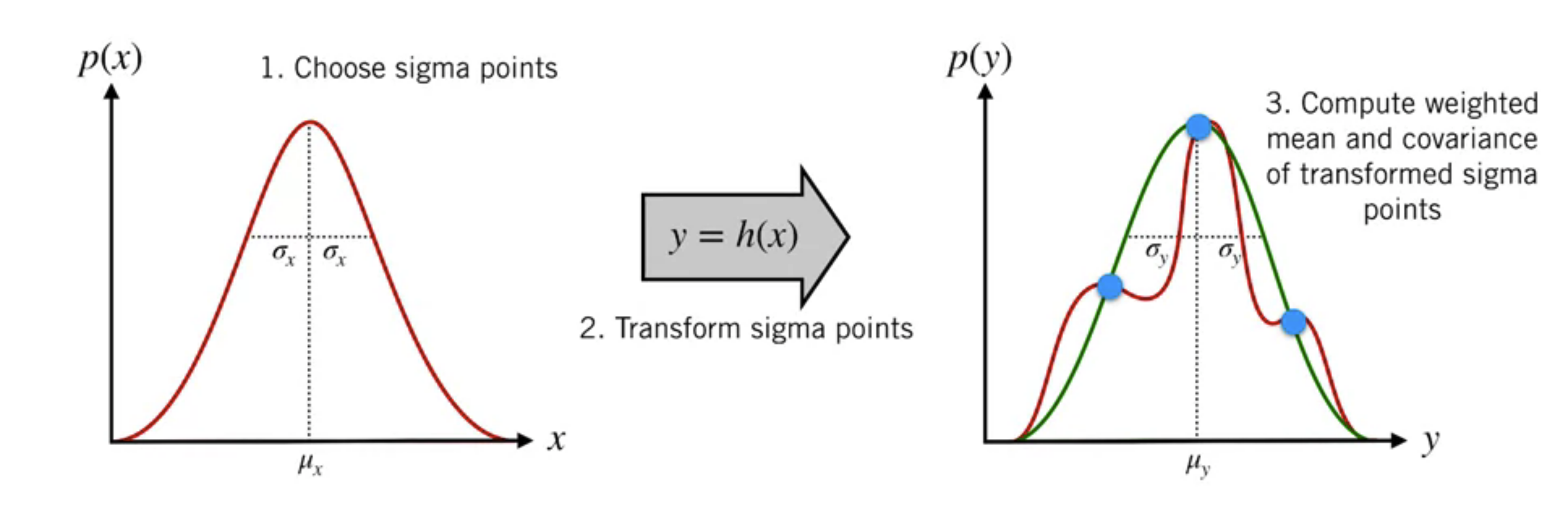
We perform a nonlinear transformation $h(x)$ on the 1D gaussian distribution (left), the result is a more complicated 1D distribution (right). We already know the mean and the standard deviation of the input gaussian, and we want to figure out the mean and standard deviation of the output distribution using this information and the nonlinear function.

UKF gives us a way to do this ny three steps

1. Choose sigma points from our input distribution

   

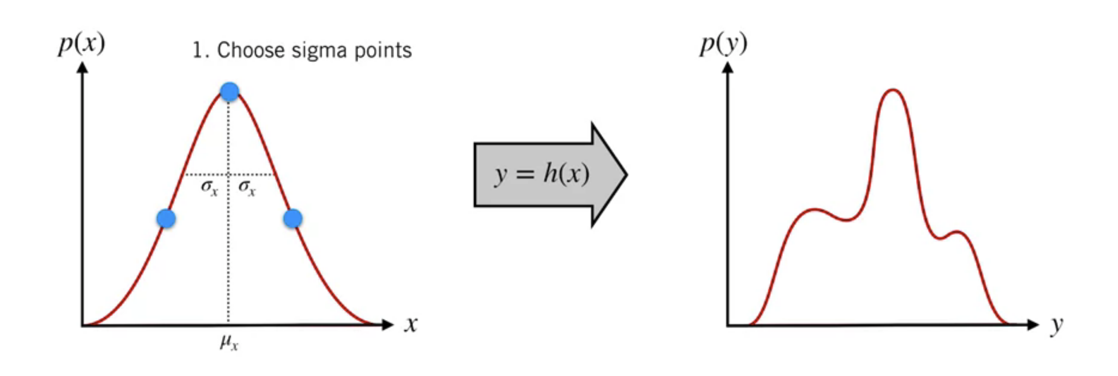
2. Transform sigma points

   

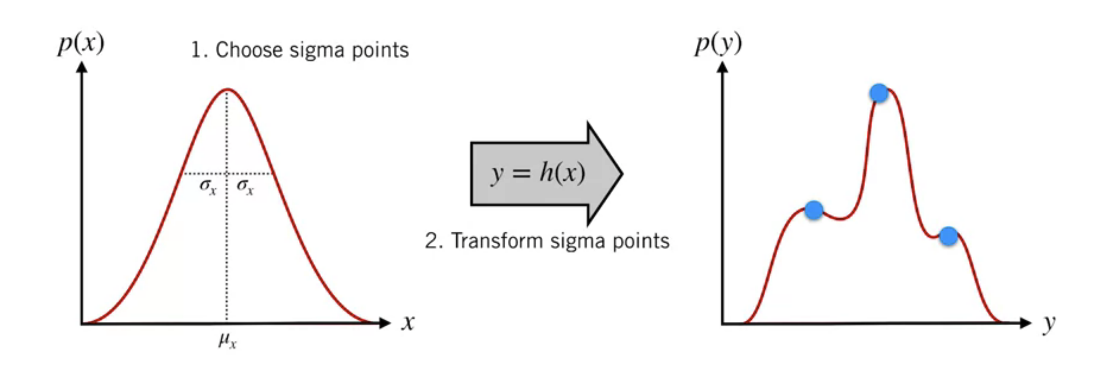
3. Compute weighted mean and covariance of transformed sigma points, which will give us a good approximation of the true output distribution.

   

Unscented Transform

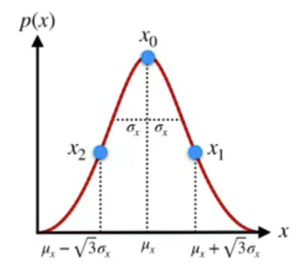
Choosing sigma points

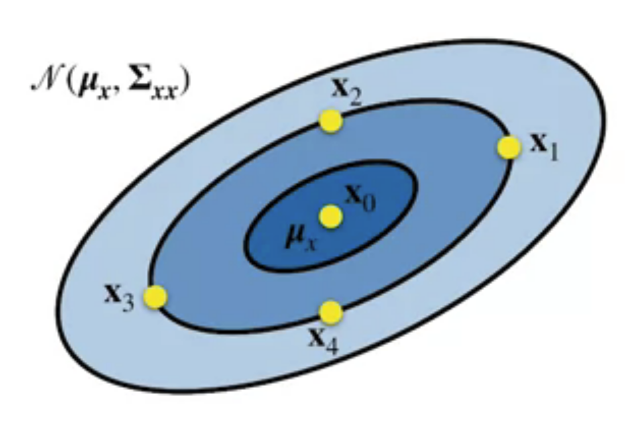
For an $N$-dimensional PDF $\mathcal{N}\left(\mu_{x}, \Sigma_{x x}\right)$ , we need $2N+1$ sigma points

• One for the mean
• and the rest symmetrically distributed about the mean

1D:

2D:

Steps

1. Compute the Cholesky Decomposition of the covariance matrix

   $$ \mathbf{L} \mathbf{L}^{T}=\boldsymbol{\Sigma}_{x x} $$

2. Calculate the sigma points

   $$ \begin{aligned} \mathbf{x}_{0} &=\boldsymbol{\mu}_{x} & & \\ \mathbf{x}_{i} &=\boldsymbol{\mu}_{x}+\sqrt{N+\kappa} \operatorname{col}_{i} \mathbf{L} & & i=1, \ldots, N \\ \mathbf{x}_{i+N} &=\boldsymbol{\mu}_{x}-\sqrt{N+\kappa} \operatorname{col}_{i} \mathbf{L} & & i=1, \ldots, N \end{aligned} $$
   • $\kappa$: tuning parameter. for Gaussian PDFs, setting $\kappa = 3 - N$ is a good choice.

Transforming

Pass each of the $2N + 1$ sigma points through the nonlinear function $\mathbf{h}(x)$

$$ \mathbf{y}_{i}=\mathbf{h}\left(\mathbf{x}_{i}\right) \quad i=0, \ldots, 2 N $$

Recombining

Compute the mean and covariance of the output PDF

• mean

  $$ \boldsymbol{\mu}_{y}=\sum_{i=0}^{2 N} \alpha_{i} \mathbf{y}_{i} $$

• covariance

  $$ \boldsymbol{\Sigma}_{y y}=\sum_{i=0}^{2 N} \alpha_{i}\left(\mathbf{y}_{i}-\boldsymbol{\mu}_{y}\right)\left(\mathbf{y}_{i}-\boldsymbol{\mu}_{y}\right)^{T} $$

with weights

$$ \alpha_{i}=\left\{\begin{array}{lr} \frac{\kappa}{N+\kappa} & i=0 \\ \frac{1}{2} \frac{1}{N+\kappa} & \text { otherwise } \end{array}\right. $$

Example

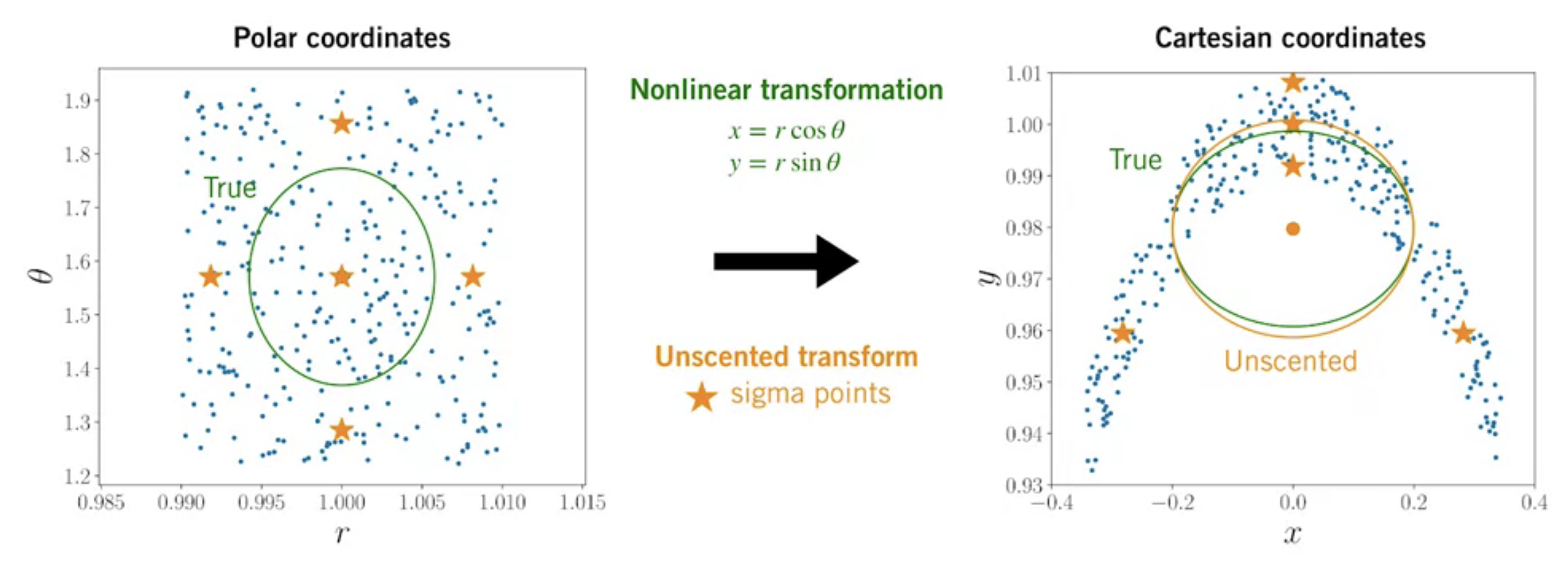
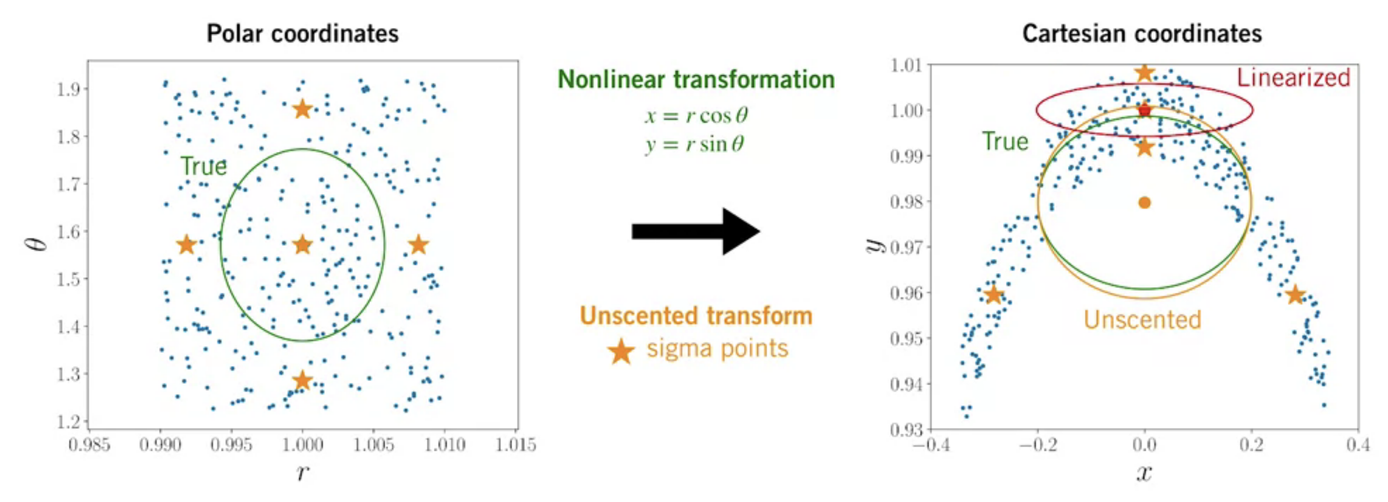
Compared to linearization (red), we can see the unscented transform (orange) gives a much better approximation!

The Unscented Kalman Filter (UKF)

💡Idea: Instead of approximating the system equations by linearizing, we will calculate sigma points and use the Unscented Transform to approxiamte the PDFs directly.

Prediction step

To propagate the state from time $k-1$ to time $k$, apply the Unscented Transform using the current best guess for the mean and covariance.

1. Compute sigma points

   $$ \begin{array}{rlrl} \hat{\mathbf{L}}_{k-1} \hat{\mathbf{L}}_{k-1}^{T} & =\hat{\mathbf{P}}_{k-1} & (\text{Cholesky Decomposition})& \\ \hat{\mathbf{x}}_{k-1}^{(0)} & =\hat{\mathbf{x}}_{k-1} & & \\ \hat{\mathbf{x}}_{k-1}^{(i)} & =\hat{\mathbf{x}}_{k-1}+\sqrt{N+\kappa} \operatorname{col}_{i} \hat{\mathbf{L}}_{k-1} & i=1 \ldots N \\ \hat{\mathbf{x}}_{k-1}^{(i+N)} & =\hat{\mathbf{x}}_{k-1}-\sqrt{N+\kappa} \operatorname{col}_{i} \hat{\mathbf{L}}_{k-1} & i=1 \ldots N \end{array} $$

2. Propagate sigma points

   $$ \breve{\mathbf{x}}_{k}^{(i)}=\mathbf{f}_{k-1}\left(\hat{\mathbf{x}}_{k-1}^{(i)}, \mathbf{u}_{k-1}, \mathbf{0}\right) \quad i=0 \ldots 2 N $$

3. Compute predicted mean and covariance (under the assumption of additive noise)

   $$ \begin{aligned} \alpha^{(i)} &=\left\{\begin{array}{ll} \frac{\kappa}{N+\kappa} & i=0 \\ \frac{1}{2} \frac{1}{N+\kappa} & \text { otherwise } \end{array}\right.\\\\ \check{\mathbf{x}}_{k} &=\sum_{i=0}^{2 N} \alpha^{(i)} \check{\mathbf{x}}_{k}^{(i)} \\\\ \check{\mathbf{P}}_{k} &=\sum_{i=0}^{2 N} \alpha^{(i)}\left(\check{\mathbf{x}}_{k}^{(i)}-\check{\mathbf{x}}_{k}\right)\left(\check{\mathbf{x}}_{k}^{(i)}-\check{\mathbf{x}}_{k}\right)^{T}+\mathbf{Q}_{k-1} \end{aligned} $$

Correction step

To correct the state estimate using measurement at time $k$, use the nonlinear measurement model and the sigma points from the prediction step to predict the measurements.

1. Predict measurements from propagated sigma points

   $$ \hat{\mathbf{y}}_{k}^{(i)}=\mathbf{h}_{k}\left(\check{\mathbf{x}}_{k}^{(i)}, \mathbf{0}\right) \quad i=0 \ldots 2 N $$

2. Estimate mean and covariance of predicted measurements

   $$ \begin{array}{l} \hat{\mathbf{y}}_{k}=\displaystyle \sum_{i=0}^{2 N} \alpha^{(i)} \hat{\mathbf{y}}_{k}^{(i)} \\ \mathbf{P}_{y}=\displaystyle\sum_{i=0}^{2 N} \alpha^{(i)}\left(\hat{\mathbf{y}}_{k}^{(i)}-\hat{\mathbf{y}}_{k}\right)\left(\hat{\mathbf{y}}_{k}^{(i)}-\hat{\mathbf{y}}_{k}\right)^{T}+\mathbf{R}_{k} \end{array} $$

3. Compute cross-covariance and Kalman Gain

   $$ \begin{aligned} \mathbf{P}_{x y} &=\sum_{i=0}^{2 N} \alpha^{(i)}\left(\check{\mathbf{x}}_{k}^{(i)}-\check{\mathbf{x}}_{k}\right)\left(\hat{\mathbf{y}}_{k}^{(i)}-\hat{\mathbf{y}}_{k}\right)^{T} \\\\ \mathbf{K}_{k} &=\mathbf{P}_{x y} \mathbf{P}_{y}^{-1} \end{aligned} $$

4. Compute corrected mean and covariance

   $$ \begin{array}{l} \hat{\mathbf{x}}_{k}=\check{\mathbf{x}}_{k}+\mathbf{K}_{k}\left(\mathbf{y}_{k}-\hat{\mathbf{y}}_{k}\right) \\ \hat{\mathbf{P}}_{k}=\check{\mathbf{P}}_{k}-\mathbf{K}_{k} \mathbf{P}_{y} \mathbf{K}_{k}^{T} \end{array} $$

UKF Example

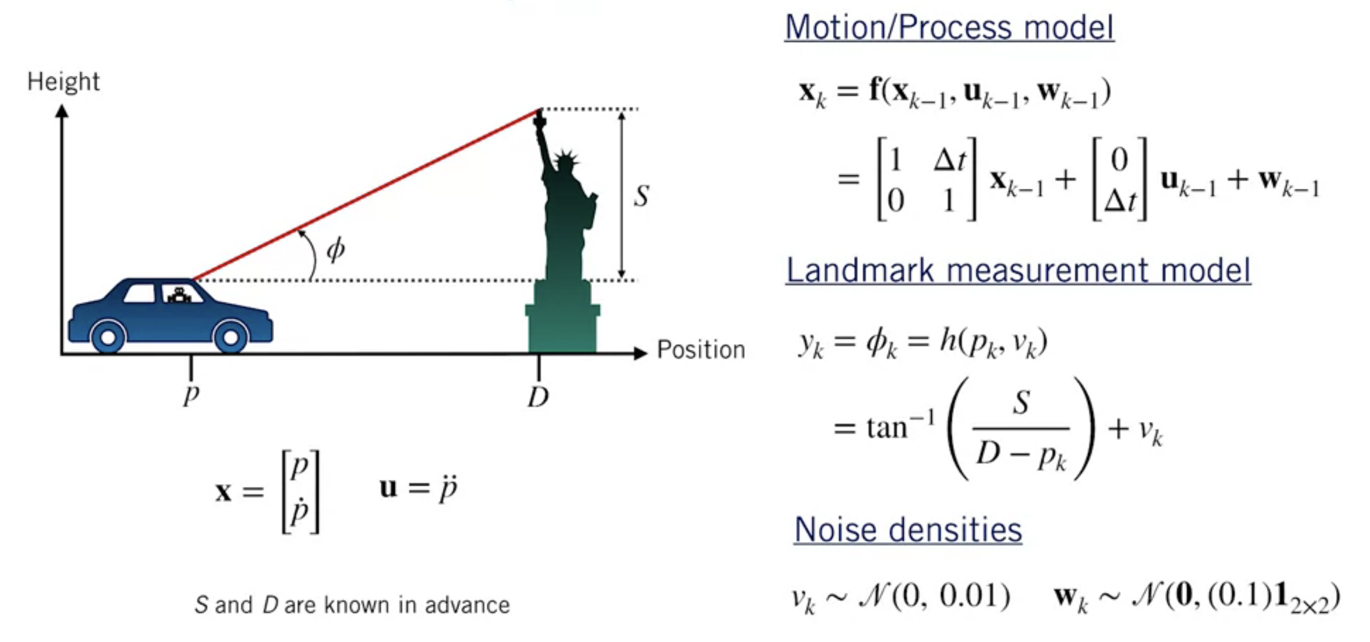
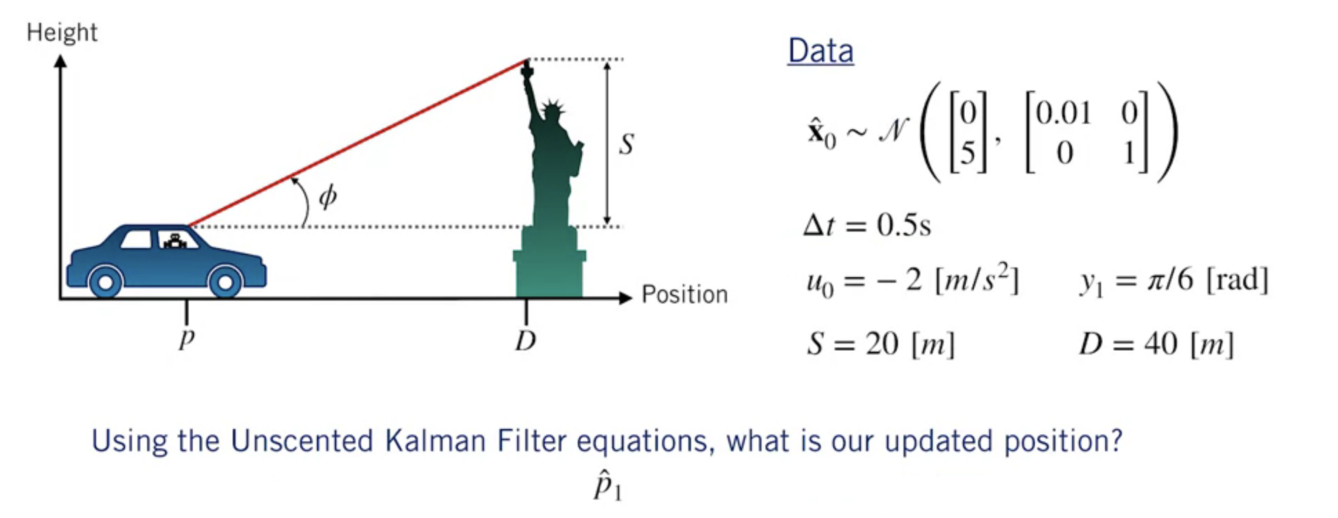
Prediction step

2D state estimate $\Rightarrow N=2, \quad \kappa=3-N=1$

1. Compute sigma points

   $$ \begin{aligned} &\hat{\mathbf{L}}_{0} \hat{\mathbf{L}}_{0}^{T}=\hat{\mathbf{P}}_{0} \\ &{\left[\begin{array}{cc} 0.1 & 0 \\ 0 & 1 \end{array}\right]\left[\begin{array}{cc} 0.1 & 0 \\ 0 & 1 \end{array}\right]^{T}=\left[\begin{array}{cc} 0.01 & 0 \\ 0 & 1 \end{array}\right]} \end{aligned} $$ $$ \begin{aligned} \hat{\mathbf{x}}_{0}^{(0)} &=\hat{\mathbf{x}}_{0} \\ \hat{\mathbf{x}}_{0}^{(i)} &=\hat{\mathbf{x}}_{0}+\sqrt{N+\kappa} \operatorname{col}_{i} \hat{\mathbf{L}}_{0} \quad i=1 \ldots, N \\ \hat{\mathbf{x}}_{0}^{(i+N)} &=\hat{\mathbf{x}}_{0}-\sqrt{N+\kappa} \operatorname{col}_{i} \hat{\mathbf{L}}_{0} \quad i=1, \ldots, N \\ \hat{\mathbf{x}}_{0}^{(0)} &=\left[\begin{array}{l} 0 \\ 5 \end{array}\right] \\ \hat{\mathbf{x}}_{0}^{(1)} &=\left[\begin{array}{l} 0 \\ 5 \end{array}\right]+\sqrt{3}\left[\begin{array}{c} 0.1 \\ 0 \end{array}\right]=\left[\begin{array}{c} 0.2 \\ 5 \end{array}\right] \\ \hat{\mathbf{x}}_{0}^{(2)} &=\left[\begin{array}{l} 0 \\ 5 \end{array}\right]+\sqrt{3}\left[\begin{array}{c} 0 \\ 1 \end{array}\right]=\left[\begin{array}{c} 0 \\ 6.7 \end{array}\right] \\ \hat{\mathbf{x}}_{0}^{(3)} &=\left[\begin{array}{l} 0 \\ 5 \end{array}\right]-\sqrt{3}\left[\begin{array}{c} 0.1 \\ 0 \end{array}\right]=\left[\begin{array}{c} -0.2 \\ 5 \end{array}\right] \\ \hat{\mathbf{x}}_{0}^{(4)} &=\left[\begin{array}{l} 0 \\ 5 \end{array}\right]-\sqrt{3}\left[\begin{array}{l} 0 \\ 1 \end{array}\right]=\left[\begin{array}{c} 0 \\ 3.3 \end{array}\right] \end{aligned} $$

2. Propagate sigma points

   $$ \begin{aligned} &\check{\mathbf{x}}_{1}^{(i)}=\mathbf{f}_{0}\left(\hat{\mathbf{x}}_{0}^{(i)}, \mathbf{u}_{0}, \mathbf{0}\right) \quad i=0, \ldots, 2 N \\ &\check{\mathbf{x}}_{1}^{(0)}=\left[\begin{array}{cc} 1 & 0.5 \\ 0 & 1 \end{array}\right]\left[\begin{array}{c} 0 \\ 5 \end{array}\right]+\left[\begin{array}{c} 0 \\ 0.5 \end{array}\right](-2)=\left[\begin{array}{c} 2.5 \\ 4 \end{array}\right] \\ &\check{\mathbf{x}}_{1}^{(1)}=\left[\begin{array}{cc} 1 & 0.5 \\ 0 & 1 \end{array}\right]\left[\begin{array}{c} 0.2 \\ 5 \end{array}\right]+\left[\begin{array}{c} 0 \\ 0.5 \end{array}\right](-2)=\left[\begin{array}{c} 2.7 \\ 4 \end{array}\right] \\ &\check{\mathbf{x}}_{1}^{(2)}=\left[\begin{array}{cc} 1 & 0.5 \\ 0 & 1 \end{array}\right]\left[\begin{array}{c} 0 \\ 6.7 \end{array}\right]+\left[\begin{array}{c} 0 \\ 0.5 \end{array}\right](-2)=\left[\begin{array}{c} 3.4 \\ 5.7 \end{array}\right] \\ &\check{\mathbf{x}}_{1}^{(3)}=\left[\begin{array}{cc} 1 & 0.5 \\ 0 & 1 \end{array}\right]\left[\begin{array}{c} -0.2 \\ 5 \end{array}\right]+\left[\begin{array}{c} 0 \\ 0.5 \end{array}\right](-2)=\left[\begin{array}{c} 2.3 \\ 4 \end{array}\right] \\ &\check{\mathbf{x}}_{1}^{(4)}=\left[\begin{array}{cc} 1 & 0.5 \\ 0 & 1 \end{array}\right]\left[\begin{array}{c} 0 \\ 3.3 \end{array}\right]+\left[\begin{array}{c} 0 \\ 0.5 \end{array}\right](-2)=\left[\begin{array}{c} 1.6 \\ 2.3 \end{array}\right] \end{aligned} $$

3. Compute predicted mean and covariance (under the assumption of additive noise)

   $$ \begin{aligned} \alpha^{(i)} &=\left\{\begin{array}{l} \frac{\kappa}{N+\kappa}=\frac{1}{2+1}=\frac{1}{3} \quad i=0 \\ \frac{1}{2} \frac{1}{N+\kappa}=\frac{1}{2} \frac{1}{2+1}=\frac{1}{6} \quad \text { otherwise } \end{array}\right.\\\\ \\ \check{\mathbf{x}}_{k}&=\sum_{i=0}^{2 N} \alpha^{(i)} \check{\mathbf{x}}_{k}^{(i)} \\ &=\frac{1}{3}\left[\begin{array}{c} 2.5 \\ 4 \end{array}\right]+\frac{1}{6}\left[\begin{array}{c} 2.7 \\ 4 \end{array}\right]+\frac{1}{6}\left[\begin{array}{l} 3.4 \\ 5.7 \end{array}\right]+\frac{1}{6}\left[\begin{array}{c} 2.3 \\ 4 \end{array}\right]+\frac{1}{6}\left[\begin{array}{l} 1.6 \\ 2.3 \end{array}\right]=\left[\begin{array}{c} 2.5 \\ 4 \end{array}\right] \end{aligned} $$ $$ \begin{aligned} \check{\mathbf{P}}_{k}=& \sum_{i=0}^{2 N} \alpha^{(i)}\left(\check{\mathbf{x}}_{k}^{(i)}-\check{\mathbf{x}}_{k}\right)\left(\check{\mathbf{x}}_{k}^{(i)}-\check{\mathbf{x}}_{k}\right)^{T}+\mathbf{Q}_{k-1} \\ =& \frac{1}{3}\left(\left[\begin{array}{c} 2.5 \\ 4 \end{array}\right]-\left[\begin{array}{c} 2.5 \\ 4 \end{array}\right]\right)\left(\left[\begin{array}{c} 2.5 \\ 4 \end{array}\right]-\left[\begin{array}{c} 2.5 \\ 4 \end{array}\right]\right)^{T}+\\ & \frac{1}{6}\left(\left[\begin{array}{c} 2.7 \\ 4 \end{array}\right]-\left[\begin{array}{c} 2.5 \\ 4 \end{array}\right]\right)\left(\left[\begin{array}{c} 2.7 \\ 4 \end{array}\right]-\left[\begin{array}{c} 2.5 \\ 4 \end{array}\right]\right)^{T}+\frac{1}{6}\left(\left[\begin{array}{c} 3.4 \\ 5.7 \end{array}\right]-\left[\begin{array}{c} 2.5 \\ 4 \end{array}\right]\right)\left(\left[\begin{array}{c} 3.4 \\ 5.7 \end{array}\right]-\left[\begin{array}{c} 2.5 \\ 4 \end{array}\right]\right)^{T}+\\ & \frac{1}{6}\left(\left[\begin{array}{c} 2.3 \\ 4 \end{array}\right]-\left[\begin{array}{c} 2.5 \\ 4 \end{array}\right]\right)\left(\left[\begin{array}{c} 2.3 \\ 4 \end{array}\right]-\left[\begin{array}{c} 2.5 \\ 4 \end{array}\right]\right)^{T}+\frac{1}{6}\left(\left[\begin{array}{c} 1.6 \\ 2.3 \end{array}\right]-\left[\begin{array}{c} 2.5 \\ 4 \end{array}\right]\right)\left(\left[\begin{array}{c} 1.6 \\ 2.3 \end{array}\right]-\left[\begin{array}{c} 2.5 \\ 4 \end{array}\right]\right)^{T}+\left[\begin{array}{cc} 0.1 & 0 \\ 0 & 0.1 \end{array}\right] \\ =& {\left[\begin{array}{cc} 0.36 & 0.5 \\ 0.5 & 1.1 \end{array}\right] } \end{aligned} $$

Correction step

1. Predict measurements from propagated sigma points

   

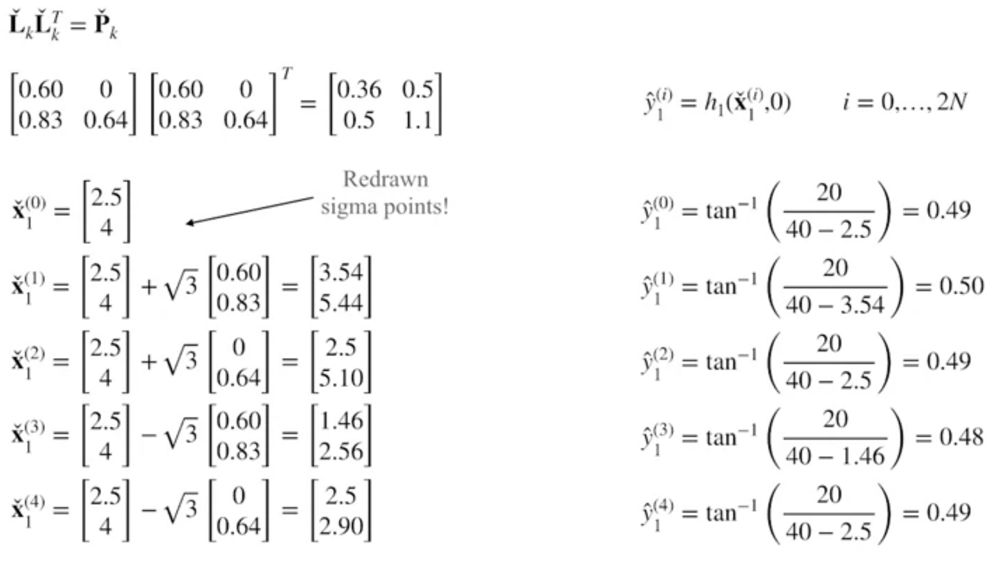
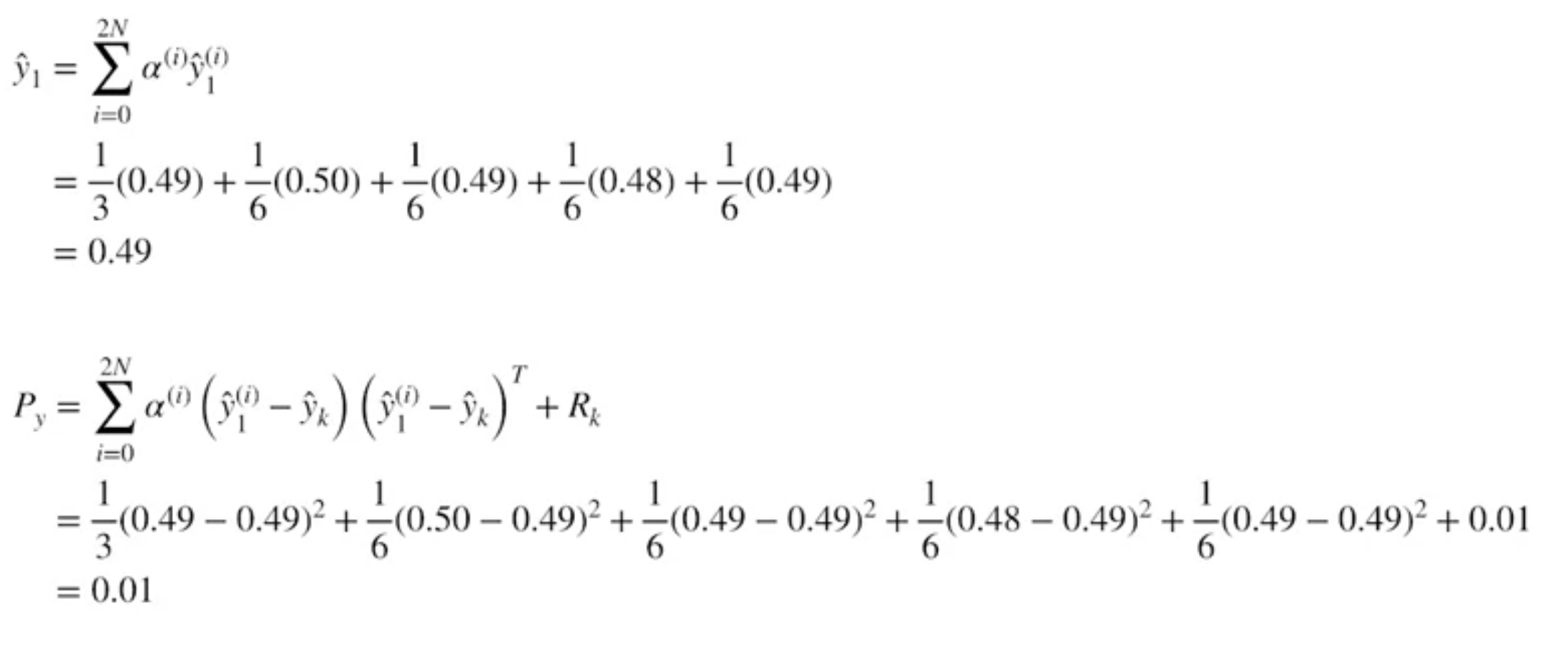
2. Estimate mean and covariance of predicted measurements

   

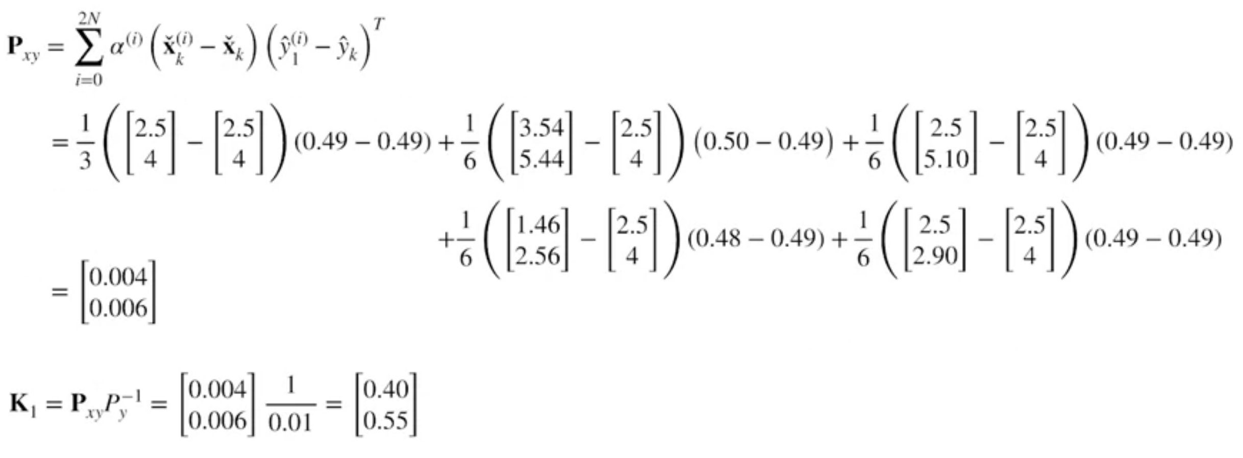
3. Compute cross-covariance and Kalman Gain

   

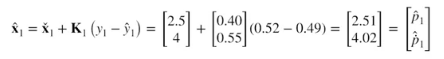
4. Compute corrected mean and covariance

   

Summary

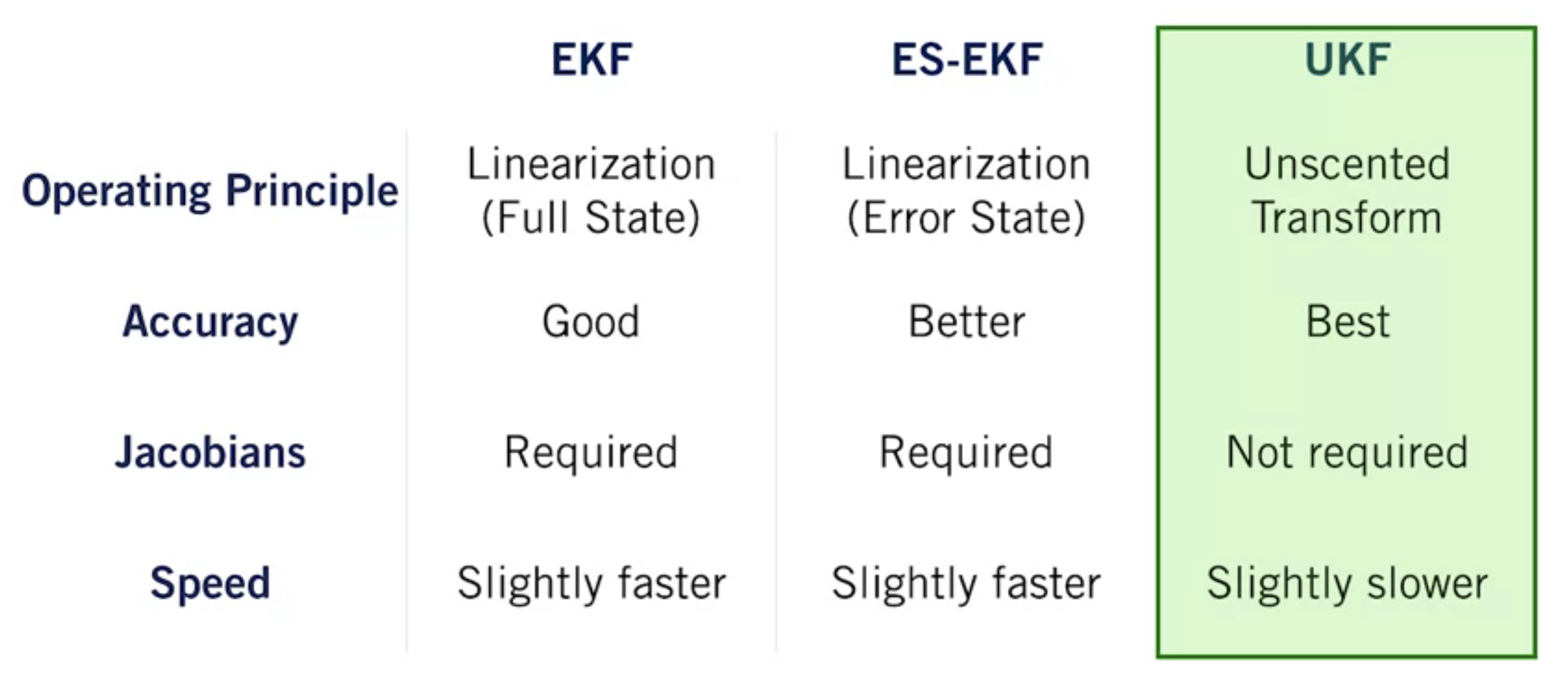
• The UKF use the unscented transform to adpat the Kalman filter to nonlinear systems.
• The unscented transform works by passing a small set of carefully chosen samples through a nonlinear system, and computing the mean and covariance of the outputs.
• The unscented transform does a better job of approixmating the output distribution than analytical local linearization, for similar computational cost

Comparision of Nonlinear KF

Reference

• An Alternative to the EKF - The Unscented Kalman Filter