Wert- und Zeitdiskrete Systeme

Vorbemerkungen

Signale in kontinuierlicher und diskreter Zeit

kontinuierliche (konti.) Zeit

Zeit ist kontinuierliche Variable
Signal $s(t)$ nimmt bestimmten Wert $s^*(t^*)$ für beliebig kurze Zeitspanne an
Zwischen zwei beliebigen Zeitpunkte $t_1$ und $t_2$ liegen unendlich viele Zeitpunkt $t_1 \leq t \leq t_2$
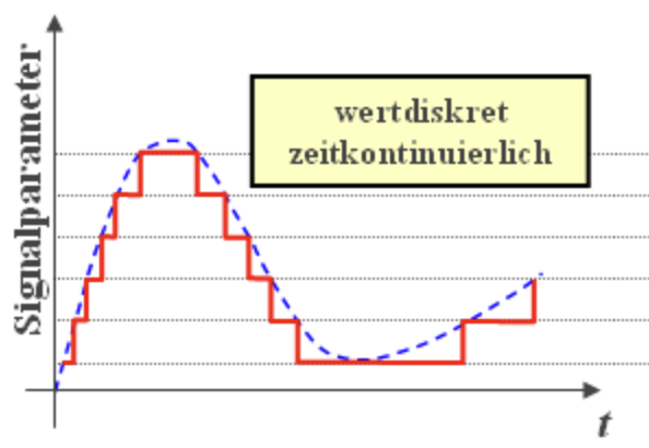
Werte könne kontinuierlich oder diskret sein

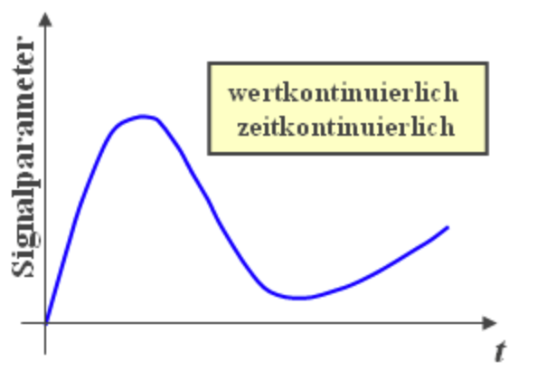
Kontinuierlich in Zeit und Wert $\rightarrow$ analoges Signal

Diskrete Zeit

Diskrete Zeitpunkt $t_k, k \in \mathbb{Z}$
$s_k := s(t_k)$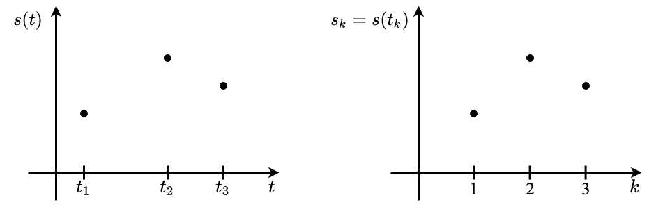
Zeitliche Anordnung der $t_k$ ist beliebig, aber in viele Fällen äquidistant
$t_k = k \cdot \Delta \quad k \in \mathbb{Z}$
Wert können kontinuierlich oder diskret sein
- Diskret in Zeit und Ort $\rightarrow$ digitales Signal
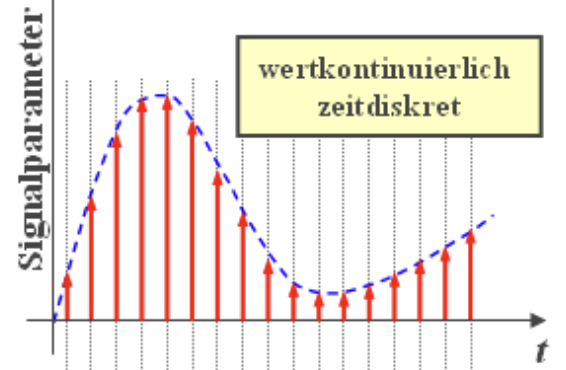
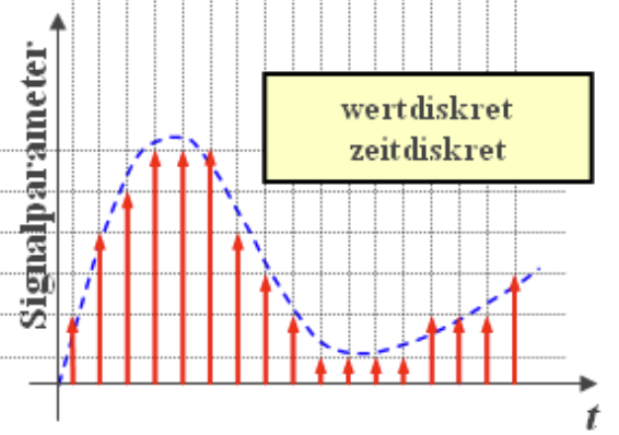
Signale können inhärent zeitdiskret sein, oder aus Abtastung kontinuierliche Signale entstehen.

Kategoriale und Kardinale Variablen

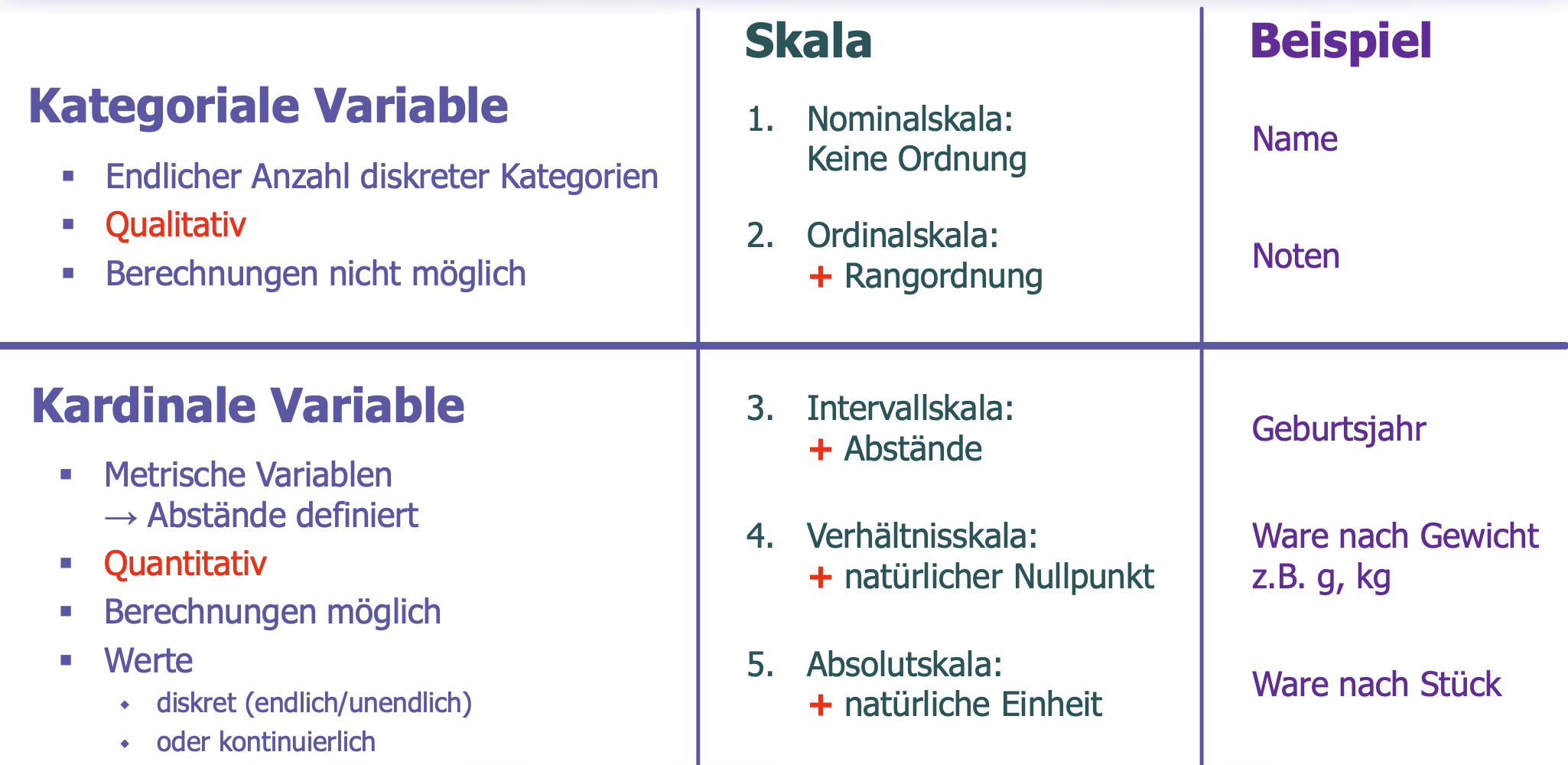
Kategoriale Variable

Nominal

The nominal scale is made up of pure labels.
- The only meaningful question to ask is whether two variables have the same value: the nominal scale only allows to compare two values w.r.t. equivalence.
- There is no meaningful transformation besides relabeling.
- No empirical operation is permissible, i.e., there is no mathematical operation of nominal features that is also meaningful in the material world.
A typical example is the sex of a human.
- The two possible values can be either written as “f” vs. “m,” “female” vs. “male”. The labels are different, but the meaning is the same.
Although nominal values are sometimes represented by digits, one must not interpret them as numbers.
- For example, the postal codes used in Germany are digits, but there is no meaning in, e.g., adding two postal codes.
- Similarly, nominal features do not have an ordering, i.e., the postal code 12345 is not “smaller” than the postal code 56789. Of course, most of the time there are options for how to introduce some kind of lexicographic sorting scheme, but this is purely artificial and has no meaning for the underlying objects. With respect to statistics, the permissible average is not the mean (since summa- tion is not allowed) or the median (since there is no ordering), but the mode, i.e., the most common value in the dataset.

Ordinal

The ordinal scale allows comparing values w.r.t. equivalence and rank.
- Any transformation of the domain must preserve the order, which means that the transformation must be strictly increasing.
- But there is still no way to add an offset to one value in order to obtain a new value or to take the difference between two values.
Example: school grades.
- In the German grading system, the grade 1 (“excellent”) is better than 2 (“good”), which is better than 3 (“satisfactory”) and so on.
  - But quite surely the difference in a student’s skills is not the same between the grades 1 and 2 as between 2 and 3, although the “difference” in the grades is unity in both cases.
  - In addition, teachers often report the arithmetic mean of the grades in an exam, even though the arithmetic mean does not exist on the ordinal scale. In consequence, it is syntactically possible to compute the mean, even though the result, e.g., 2.47 has no place on the grading scale, other than it being “closer” to a 2 than a 3. The Anglo-Saxon grading system, which uses the letters “A” to “F”, is somewhat immune to this confusion.
The correct average involving an ordinal scale is obtained by the median.

Kardinale Variable

Interval

The interval scale allows adding an offset to one value to obtain a new one, or to calculate the difference between two values—hence the name.
However, the interval scale lacks a naturally defined zero. Values from the interval scale are typically represented using real numbers, which contains the symbol “0,” but this symbol has no special meaning and its position on the scale is arbitrary. For this reason, the scalar multiplication of two values from the interval scale is meaningless. Permissible transformations preserve the order, but may shift the position of the zero.

Verhältnis

The ratio scale has a well defined, non-arbitrary zero, and therefore allows calculating ratios of two values.
- This implies that there is a scalar multiplication and that any transformation must preserve the zero.
Many features from the field of physics belong to this category and any transformation is merely a change of units.

Absolut

The absolute scale shares these properties, but is equipped with a natural unit and features of this scale can NOT be negative. In other words, features of the absolute scale represent counts of some quantities. Therefore, the only allowed transformation is the identity.

Wertdiskrete Systeme

Statische Systeme

Ein-/Ausgang: Zufallsvariable $u_k$ (Eingang) und $y_k$ (Ausgang), $k \in \mathbb{N}_0$

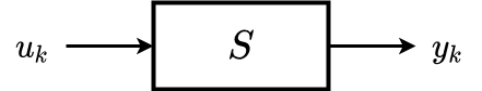
wertdiskrete_systeme-statistische_systeme.drawio

$u_k$ und $y_k$ sind wertdiskret, wobei o.B.d.A

\begin{array}{l} u_{k} \in\{1,2, \cdots, p\} \\ y_{k} \in\{1,2, \ldots, M\} \end{array}

Stochastische Abhängigkeit $y_k$ von $u_k$ :

P\left(y_{k}=i \mid u_{k}=j\right) \qquad j \in\{1, \cdots, p\}, i \in\{1, \ldots, m\}

Anordnung der Wahrscheinlichkeit in Matrix $A_k$ :

\mathbf{A}_{k}=\left(\begin{array}{ccc} P\left(y_{k}=1 \mid u_{k}=1\right) & \cdots & P\left(y_{k}=M \mid u_{k}=1\right) \\ \vdots & & \vdots \\ P\left(y_{k}=1 \mid u_{k}=P\right) & \cdots & P\left(y_{k}=M \mid u_{k}=P\right) \end{array}\right)

Elemente $\geq 0$
Zeilensumme $= 1$
Auftrittswahrscheinlichkeit als Vektoren:
$\eta_{k}^{u}=\left(\begin{array}{c} P\left(u_{k}=1\right) \\ P\left(u_{k}=2\right) \\ \vdots \\ P\left(u_{k}=P\right) \end{array}\right) \qquad \eta_{k}^{y}=\left(\begin{array}{c} P\left(y_{k}=1\right) \\ P\left(y_{k}=2\right) \\ \vdots \\ P\left(y_{k}=M\right) \end{array}\right)$

Berechnung von $\eta_k^y$ aus $\eta_k^u$ (in Vektor-Matrix-Form):

\eta_{k}^{y}=\mathbf{A}_{k}^{\top} \eta_{k}^{u}

Details

\begin{aligned} P\left(y_{k}=i\right) &=\sum_{j=1}^{P} P\left(y_{k}=i, u_{k}=j\right) \\\\ &=\sum_{j=1}^{p} P\left(y_{k}=i \mid u_{k}=j\right) \cdot P\left(u_{k}=j\right) \end{aligned}

Spezialfall: $u_k = j^*$ ist bekannt, also

\begin{array}{l} P\left(u_{k}=j^{*}\right)=1 \\ P\left(u_{k}=j\right)=0 \quad j=1, \cdots M, j \neq j^{*} \end{array}

\begin{aligned} \Rightarrow \quad P\left(y_{k}=i\right) &=\sum_{j=1}^{p} p\left(y_{k}=i \mid u_{k}=j\right) P\left(u_{k}=j\right) \\ &=P\left(y_{k}=i \mid u_{k}=j^{*}\right) \end{aligned}

In Vektor-Matrix-Form:

\eta_{k}^{y}={\underbrace{\mathbf{A}_{k}\left(j^{*}, :\right)}_{\text{die } j^*-\text{te Zeile von } A_k}}^\top=\left(P\left(y_{k}=1 \mid u_{k}=j^{*}\right) \cdots P\left(y_{k}=M \mid u_{k}=j^{*}\right)\right)^{\top}

Dynamische Systeme

Der aktuellen Ausgang $y_k$ ist abhängig von
- dem aktuellen Eingang $u_k$
- dem aktuellen Zustand $x_k$
Aufteilung des dynamischen Systems in zwei Teile
- Systemabbildung (dynamischer Teil): beschreibt zeitliche Entwicklung des Zustands $x_k$
- Messabbildung (statischer Teil): beschreibt die Abbildung des Ausgang $y_k$ von Zustand $x_k$ (und evtl. von aktuellem Eingang $u_k$ )

Systemabbildung

Zufallsvariable $x_k, k \in \mathbb{N}_0$ mit $x_k \in \{1, 2, \dots, N\}$
Entwicklung des Zustands $x_k$ bescrhieben ducrch
$P(x_{k+1}=i | x_k, \dots, x_1, x_0, u_k)$
( $u_k$ oft explizit forgelassen)

Definition

Bei $x_k$ handelt es sich um eine Markov-Ketter (erster Ordnung), falls gilt

P\left(x_{k+1}=i \mid x_{k}, \ldots, x_{1}, x_{0}, u_{k}\right)=P\left(x_{k+1}=i \mid x_{k}, u_{k}\right)

Die zukünftige Entwicklung $x_{k+1}$ ist bedingt unabhängig von vergangen Zuständen $x_{k-1}, \dots, x_1, x_0$ , falls aktueller Zustand $x_k$ bekannt ist
Vereinfachte Übergangswahrscheinlichkeit
$P(x_{k+1} = j| x_k = i)$

Definition

Eine Markov-Kette wird als Zeithomogen oder allg. als zeitinvariant bezeichnet, falls die Übergangswahrscheinlichkeit nicht von Zeitindex abhängen, d.h. es gilt

P\left(x_{k+1}=j \mid x_{k}=i\right)=\mathbf{A}(i, j)

Übergangsmatrix (zeithomogen):

\mathbf{A}=\left(\begin{array}{cccc} A(1,1) & A(1,2) & \ldots & A(1, N) \\\\ A(2,1) & A(2,2) & \cdots & A(2, N) \\\\ \vdots & \vdots & & \vdots \\\\ A(N, 1) & A(N, 2) & \cdots & A(N, N) \end{array}\right)

Definition

Eine quadratische Matrix $\mathbf{A}$ heißt Markov-Matrix, falls

Alle Elemente nicht-negative sind
$A(i, j) \geq 0 \quad \text{ für } i, j \in \\{1, \dots, N\\}$
Die Zeilensumme gleich 1
$\sum_{i=1}^{N} A(i, j)=1 \quad \text{für } i \in \\{1, \dots, N\\}$

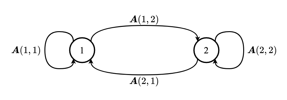
Graphische Darstellung einer Markov-Kette:

z.B. $N=2, x_k \in \\{1, 2\\}$

wertdiskrete_systeme-Markov_Kette.drawio

Messabbildung

Zustand typischerweise NICHT direkt verfügbar (latente Variable)
Messabbildung vom Zustand $x_k$ und dem aktuelle Eingang $u_k$ auf aktuelle Ausgang $y_k$
$P\left(y_{k}=j \mid x_{k}=i, u_{k}=m\right)$
- $u_k$ oft explizit forgelassen
Zeithomogen (allg. zeitinvariant)
$P\left(y_{k}=j|x_{k}=i\right)=B(i, j)$
Messe-/Beobachtungsmatrix
$\mathbf{B}=\left[\begin{array}{ccc} B(1,1) & \cdots & B(1, M) \\ \vdots & & \vdots \\ B(N, 1) & \cdots & B(N, M) \end{array}\right]$

Gesamtes Dynamisches System

Hidden Markov Model

Zustand
- Wert $x_k, k=1,2,\dots$
- Verteilung $\eta_k^x, k=1,2,\dots$
Initialer Zustand
- Wert $x_0$
- Verteilung $\eta_0^x$
Eingänge
- Werte $u_k, k=0,1,\dots$
- Verteilung $\eta_k^u,k=0,1,\dots$
Ausgänge
- Werte $y_k, k=0,1,\dots$
- Verteilung $\eta_k^y,k=0,1,\dots$
Systemabbildung $\mathbf{A}_k$
Messabbildung $\mathbf{B}_k$

Graphische Darstellung

Ausgerollte zeitliche Abhängigkeit der Zufallsvariablen
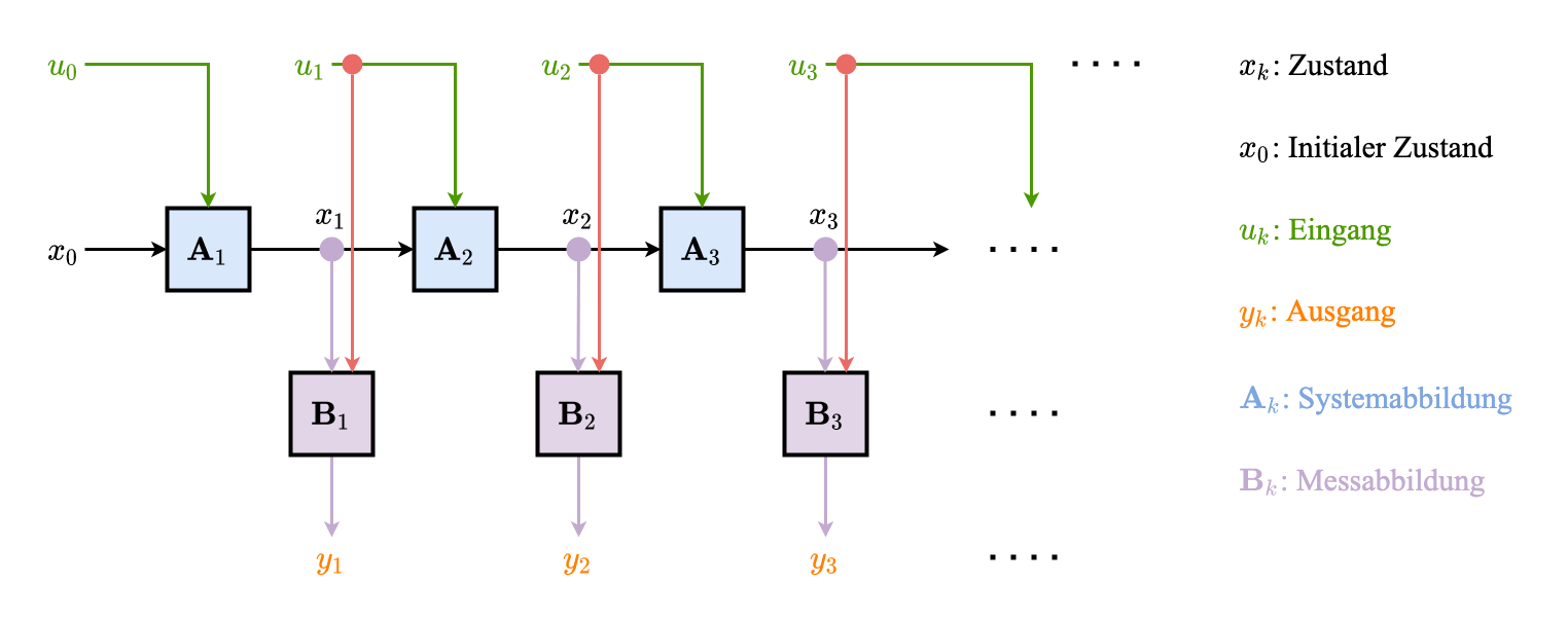
Markot-Kette (ausgerollte Darstellung)
Rekursive Darstellung der zeitliche Abbildung der Zufallsvariablen
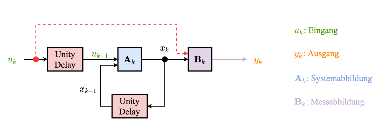
Markot-Kette (rekursive Darstellung)
Betont Übergange und Wahrscheinlichkeit
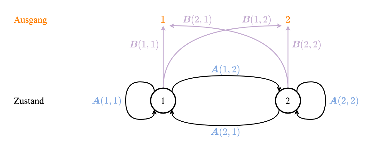
Markot-Kette (betont Übergange und Wahrscheinlichkeit)

Last updated on 2024-09-07

Zustandsschätzung 2022-06-08 →