Berechnung der Momente: Unscented Kalman Filter (UKF)
Analytische Momente
- Scheinbar die beste Methode, da schnell & feste Laufzeit 👍
- Aber
- Herleitung aufwändig
- Formeln werden schnell unhandlich groß
Beispiel: Kubisches Sensorproblem (skalar)
Output $y$ ist nonlinear abhängig von dem Zustand $x$:
$$ y=h(x)+v=x^{3}+v $$Gegeben
- Priore Schätzung $x_p \sim \mathcal{N}(\hat{x}_p, \sigma_p^2)$
- Messung $\hat{y}$
- Rauschen $v$ ist Gaußverteilt mit $E\{v\}=0, \operatorname{Cov}\{v\}=Z_{v}^{2}$
Definiere
$$ z := \left[\begin{array}{l} x \\ y \end{array}\right] \Rightarrow E\{\underline{z}\}=\left[\begin{array}{c} \hat{x}_{p} \\ E\{h(x)\} \end{array}\right] $$mit
$$ E\{h(x)\}=\int_{\mathbb{R}} h(x) f_{p}(x) d x=\int_{\mathbb{R}} x^{3} f_{p}(x) d x=\hat{x}_{p}^{2}+3 \hat{x}_{p} \sigma_{p}^{2}=:E_{3} $$Definiere
$$ \bar{h}(x)=h(x)-E\{h(x)\} $$Dann
$$ \operatorname{Cov}\{\underline{z}\}=\left[\begin{array}{ll} \mathbf{C}_{x x} & \mathbf{C}_{x y} \\ \mathbf{C}_{y x} & \mathbf{C}_{y y} \end{array}\right]=\left[\begin{array}{cc} \sigma_{p}^{2} & E\left\{\left(x-\hat{x}_{p}\right) \bar{h}(x)\right\} \\ E\left\{\left(x-\hat{x}_{p}\right) \bar{h}(x)\right\} & E\left\{\overline{h}^{2}(x)\right\}+\sigma_{v}^{2} \end{array}\right] $$ $$ \begin{aligned} E\left\{\left(x-\hat{x}_{p}\right)\bar{h}(x)\right\} &= E\left\{\left(x-\hat{x}_{p}\right)\left(x^{3}-E_{3}\right)\right\} \\ &= E\left\{x^{4}-\hat{x}_{p} x^{3}-E_{3} x+\hat{x}_{p} E_{3}\right\} \\ &= E_4 - \hat{x}_p E_3 - E_3 \hat{x}_p + \hat{x}_p E_3 \\ &= E_4 - \hat{x}_p E_3 \end{aligned} $$mit
$$ \begin{aligned} E_{q}&=\hat{x}_{p}^{4}+6 \hat{x}_{p}^{2} \sigma_{p}^{2}+3\sigma_{p}^{4} \\\\ &=\hat{x}_{p}^{4}+6 \hat{x}_{p}^{2} 2_{p}^{2}+3\sigma_{p}^{4}-\hat{x}_{p}^{4}-3 \hat{x}_{p}^{2} \sigma_{p}^{2} \\\\ &=3 \sigma_{p}^{4}+3 \hat{x}_{p}^{2} \sigma_{p}^{2} \\\\ &=3\sigma_{p}^{2}\left(\hat{x}_{p}^{2}+2_{p}^{2}\right) \end{aligned} $$und
$$ E\left\{\bar{h}^{2}(x)\right\}=9 \hat{x}_{p}^{4} \sigma_{p}^{2}+36 \hat{x}_{p}^{2} \sigma_{p}^{4}+15\sigma_{p}^{6} $$In der Kalmanfilter Filterungsgleichung einsetzen ergibt sich
$$ \begin{array}{l} \hat{x}_{e}=\hat{x}_{p}+\mathbf{C}_{xy}\mathbf{C}_{yy}^{-1}(\hat{y}-E\{h(x)\}) \overset{\text{skalar}}{=} \hat{x}_{p}+\frac{\mathbf{C}_{x y}}{\mathbf{C}_{y y}}(\hat{y}-E\{h(x)\}) \\ \sigma_{y}^{2}= \sigma_{p}^{2}-\mathbf{C}_{xy}\mathbf{C}_{yy}^{-1}\mathbf{C}_{yx} \overset{\text{skalar}}{=} \sigma_{p}^{2}-\frac{\mathbf{C}_{x y}^{2}}{\mathbf{C}_{y y}} \end{array} $$Einschub: Momente Gaußdichte
Theorem
Die zentralen Momente einer Gaußdichte sind gegeben durch
$$ C\_{i}=E\_{f}\left\\{(\boldsymbol{x}-\hat{x})^{i}\right\\}=\left\\{\begin{array}{ll} \displaystyle\prod\_{j=1, j\text{ ungeradde}}^{i-1} j \sigma^{i}=1 \cdot 3 \cdot 5 \cdots(i-1) \sigma^{i} & i \text { gerade } \\\\ 0 & i \text { ungerade } \end{array}\right. $$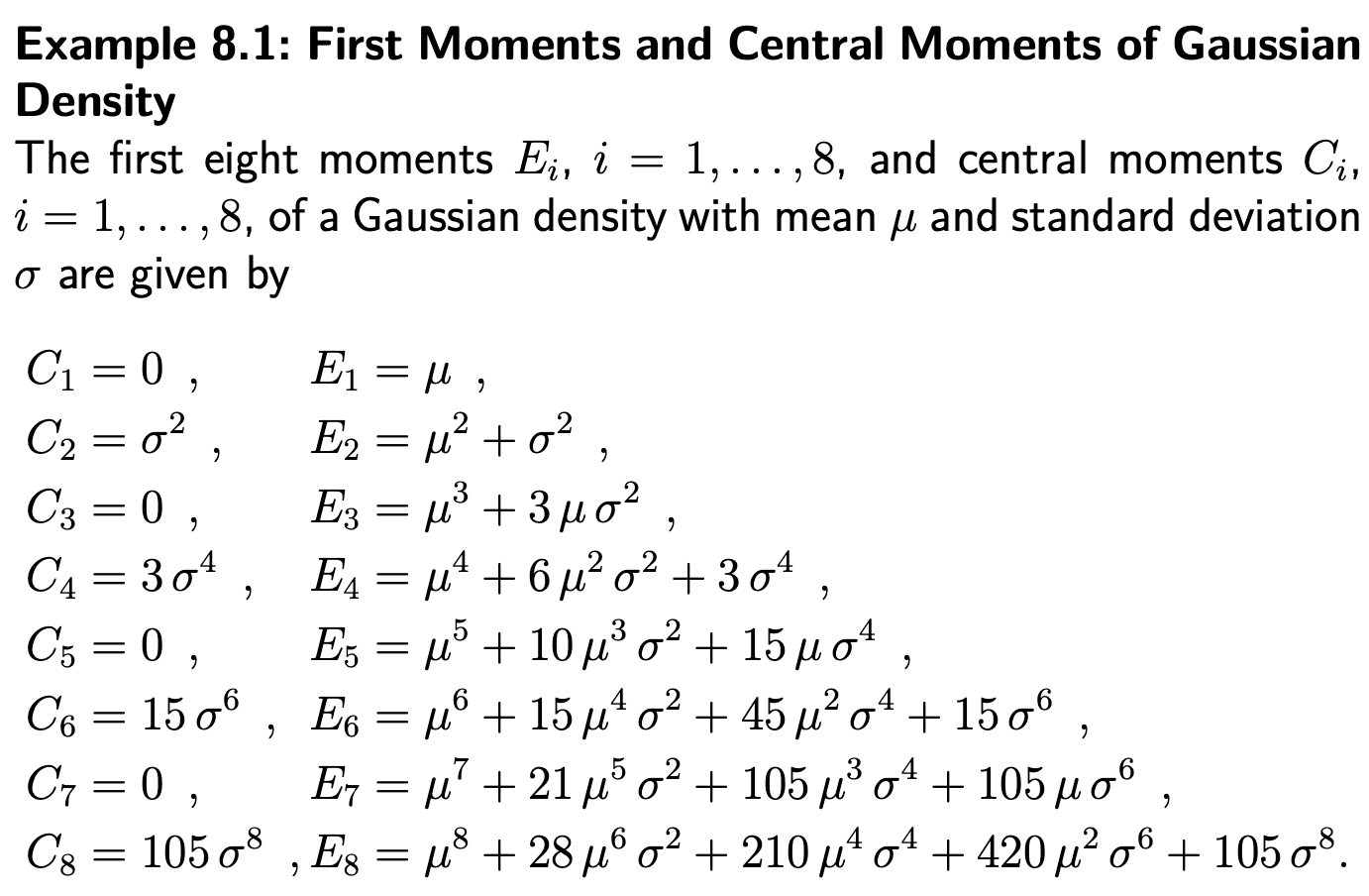
Numerische Momente
Verwendung von Standardverfahren zur Integration
👍 Vorteile
- Nutzung schneller Implementierungen
- Einstellbare Genauigkeit
- Adaptive Integration
👎 Nachteile
- Nicht für das konkrete Probleme der Momentenberechnung maßgeschneidert
Basierend auf Abtastwerten der prioren Dichte
Approximation der Prioren Gaußdichte durch Samples
Verschiedene Verfahren mit unterschiedliche Komplexität, Effizienz, Genauigkeit
Zufälliges Sampling mit Zufallszahlengenerator $\rightarrow$ unabhängige Samples
Abtastung (z.B. äquidistantes Gitter)
Minimale Approximation auf den Hauptachsen
Verwendung von $2N$ oder $2N + 1$ samples ($N$: #Dimension)
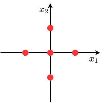
Genaue Approximation auf den Hauptachsen
Allgemeine Sample-Approximation $\rightarrow$ Systematische Approximation durch Minimierung eines Gütemaßes
Einschub: Diracsche Deltafunktion
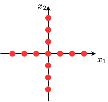
Betrachtung Grenzfall einer Gaußdichte
$$ f(x, m, \sigma)=\frac{1}{\sqrt{2 \pi} \sigma} \exp \left\{-\frac{1}{2} \frac{(x-m)^{2}}{\sigma^{2}}\right\} $$für $\sigma \rightarrow 0$
Plotting verschiedener Gaußdichte für $m=0$.
Dirasche Deltafunktion
$$ \delta(x-m)=\lim _{\sigma \rightarrow 0} f(x, m, \sigma) $$Wenn die Bereite gegen 0 ($\sigma \to 0$), die Höhe gegen unendlich.
$$ \int_{-\infty}^{\infty} \delta(x-m) d x=1 $$Definition: Diracsche Deltafunktion
$$ \delta(x)=\left\\{\begin{array}{cc} \text{Nicht definiert} & x=0 \\\\ 0 & \text { sonst } \end{array}\right. $$ $$ \int_{-\infty}^{\infty} \delta(x) d x=\int_{-\varepsilon}^{\varepsilon} \delta(x) d x=1, \varepsilon>0 $$- Laut Definition hat die Dirasche Deltafunktion alle Eigenschaften einer Dichte
- Wichtige Eigenschaften
- $f(x) \cdot \delta(x-m)=f(m) \delta(x-m)$
- $\int_{\mathbb{R}} f(x) \delta(x-m) d x=f(m)$
Heaviside Funktion (Unit Step Function)
Cumulative Verteilungsfunktion der Gaußdichte
$$ F(x)=P(\boldsymbol{x} \leq x)=\int_{-\infty}^{x} f(x) d x=\frac{1}{2}\left\{1+\operatorname{erf}\left(\frac{x-m}{\sqrt{2} \sigma}\right)\right\} $$Es gilt
$$ f(x)=\frac{d}{d x} F(x) $$Definition: Heaviside Funktion
$$ H(x-m)=\lim\_{\sigma \to 0} F(x)=\left\\{\begin{array}{ll} 1 & x>m \\\\ \frac{1}{2} & x=m \\\\ 0 & xCumulative Verteilungsfunktion von $\delta(x)$ ist $H(x)$ mit
$$ \begin{array}{l} H(x)=\displaystyle\int_{-\infty}^{x} \delta(x) d x \\\\ \delta(x)=\frac{d}{d x} H(x) \end{array} $$Multivariate Diracsche Deltafunktion
Dirasche Mischdichten (Dirac Mixture)
$$ f(x)=\sum_{i=1}^{L} \omega_{i} \delta \left(x-x_{i}\right) $$Multivariate Diracdichte
$$ \delta(\underline{x})=\delta\left(x_{1}\right) \cdot \delta\left(x_{2}\right) \cdot \ldots, \quad \underline{x}=\left[x_{1}, x_{2}, \ldots\right]^{\top} $$Multivariate Dirasche Mischdichte
$$ f(\underline{x})=\sum_{i=1}^{L} \omega_{i} \delta\left(\underline{x}-\underline{x}_{i}\right) $$Umrechnung SNV $\rightarrow$ Allgemeine Gaußdichte
(SNV = Standard Normalverteilung $\mathcal{N}(0, 1)$)
- Natürliche Lösung für Problem
- Verschiedene Möglichkeiten mit unterschiedlicher Komplexität und Effizienz
Angenommen: Wir haben ein Approximationsverfahren, das eine standardverteilung in merh-/höher-dimension approximieren kann.
- Gegeben: Gaußdichte mit $\underline{\hat{x}}=\underline{0}$ und $\mathbf{C}_x = \mathbf{I}_N$ ($N$-dim. Einheitsmatrix)
- Gesucht: Dichte mit beliebigen Mittelwert $\underline{\hat{y}}$ und Kovarianzmatrix $\mathbf{C}_y$
Wir machen Cholesky-Zerlegung
$$ \mathbf{C}_{y}=\mathcal{C}_{y} \cdot \mathcal{C}_{y}^{\top} $$wobei $\mathcal{C}_y$ eine untere Dreiecksmatrix.
Umrechnung
$$ \underline{y}=\mathcal{C}_{y} \cdot \underline{x}+\underline{\hat{y}} $$Beweis:
$$ E\{\underline{y}\}=E\left\{\mathcal{C}_{y} \cdot \underline{x}+\hat{y}\right\}=\mathcal{C}_{y} \underbrace{E\{\underline{x}\}}_{=\underline{0}}+\underbrace{E\{\hat{y}}_{=\underline{y}}\}=\underline{\hat{y}} $$ $$ \begin{aligned} \operatorname{Cov}\{\underline{y}\} &=E\left\{(\underline{y}-E\{\underline{y}\})(\underline{y}-E\{\underline{y})^{\top}\right\} \\ &=E\left\{(\underline{y}-\underline{\hat{y}})(\underline{y}-\underline{\hat{y}})^{\top}\right\} \\ &=E\left\{\mathcal{C}_{y} \cdot \underline{x} \cdot \underline{x}^{\top} \mathcal{C}_{y}^{\top}\right\}\\ &=\mathcal{C}_{y} \cdot \underbrace{E\left\{\underline{x}\underline{x}^{\top}\right\}}_{=\mathbf{C}_{x}=\mathbf{I}_{N}} \cdot \mathcal{C}{y}^{\top} \\ &=\mathcal{C}_{y} \cdot \mathbf{I}_{N} \cdot \mathcal{C}_{y}^{\top}=\mathcal{C}_{y} \cdot \mathcal{C}_{y}^{\top} = \mathbf{C}_{y} \end{aligned} $$Minimale Approximation SNV auf Hauptachsen
1D-Fall
Die wahre Dichte $\tilde{f}(x)$ sei eine 1D Standardnormalverteilung (SNV). Die möchten wir darstellen über eine Dirac Mixture
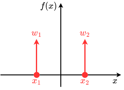 $$
f(x)=w_{1} \delta\left(x-x_{1}\right)+w_{2} \delta\left(x-x_{2}\right) \qquad w_{1}, w_{2} \geqslant 0
$$
$$
f(x)=w_{1} \delta\left(x-x_{1}\right)+w_{2} \delta\left(x-x_{2}\right) \qquad w_{1}, w_{2} \geqslant 0
$$Gaußdichte ist symmetrisch $\Rightarrow$
$$ w_{1}=w_{2}=w, \quad x_{1}=-x_{2} $$Integral soll gleich 1 sein.
$$ \int_{\mathbb{R}} f(x) d x=w_{1}+w_{2}=2 w \stackrel{!}{=} 1 \Rightarrow w=\frac{1}{2} $$Erwartungswert:
$$ E_{f}\{x\}=0=E_{\tilde{f}}\{x\} $$Varianz:
$$ E_{f}\left\{x^{2}\right\}=\int_{\mathbb{R}} x^{2} f(x) d x=w x_{1}^{2}+w x_{2}^{2}=2 w x_{1}^{2} \stackrel{!}{=} 1 \Rightarrow x_{1}^{2}=1 \Rightarrow x_1 = -1, x_2 = 1 $$2D-Fall
 $$
\begin{aligned}
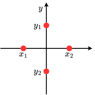
f(x, y)=& w_{1} \delta\left(x-x_{1}\right) \delta(y)+w_{2} \delta\left(x-x_{2}\right) \delta(y) & w_{1}, w_{2} \geqslant 0 \\
&+v_{1} \delta(x) \delta\left(y-y_{1}\right)+v_{2} \delta(x) \delta\left(y-y_{2}\right) & v_{1}, v_{2} \geqslant 0
\end{aligned}
$$
$$
\begin{aligned}
f(x, y)=& w_{1} \delta\left(x-x_{1}\right) \delta(y)+w_{2} \delta\left(x-x_{2}\right) \delta(y) & w_{1}, w_{2} \geqslant 0 \\
&+v_{1} \delta(x) \delta\left(y-y_{1}\right)+v_{2} \delta(x) \delta\left(y-y_{2}\right) & v_{1}, v_{2} \geqslant 0
\end{aligned}
$$Symmetrie $\Rightarrow$
$$ w_{1}=w_{2}=v_{1}=v_{2}=w, \quad x_{1}=-x_{2}, \quad v_{1}=-y_{2} $$Integral = 1
$$ \int_{\mathbb{R}^{2}} f(x, y) d x d y=w\left\{\int_{\mathbb{R}} s\left(x-x_{1}\right) d x \int_{\mathbb{R}} f(y) d y+\ldots\right\}=4 w \stackrel{!}{=} 1 \Rightarrow w=\frac{1}{4} $$Varianz
$$ \iint_{\mathbb{R}} x^{2} f(x, y) d x d y=w x_{1}^{2}+w x_{2}^{2}=2 w x_{1}^{2} \stackrel{!}{=} 1 \Rightarrow x_{1}^{2}=2 \Rightarrow x_1 = -\sqrt{2}, x_2 = \sqrt{2} $$$x, y$ sind nicht unabhänging:
$$ f(x, y) \neq f(x) \cdot f(y), E\{x \cdot y\}=0 $$N-dim Fall
$$ \begin{array}{c} w=\frac{1}{2 N} \quad \underline{x}=\left[x^{(1)}, x^{(2)}, \ldots\right]^{\top} \\ \Rightarrow \begin{equation} x_{1}^{(i)}=-\sqrt{N}, \quad x_{2}^{(i)}=+\sqrt{N}, \quad i=1, \ldots, N \end{equation} \end{array} $$Ablauf des Filters mit Sampling der prioren Dichte
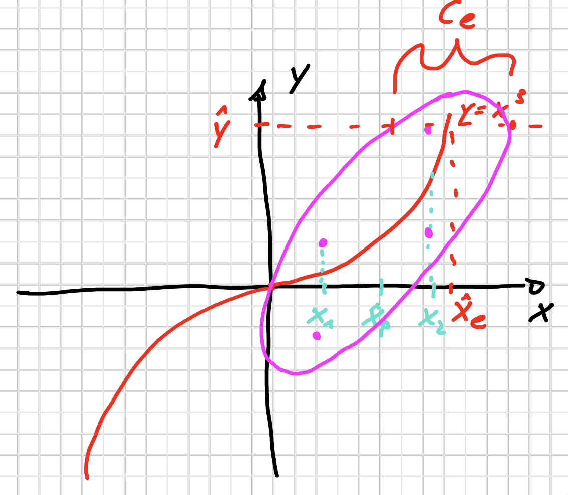
Messfunktion (Bsp.)
$$ y = x^3 + v $$Priore Schätzung: Gaußdichte $\tilde{f}_{p}(x)=\mathcal{N}\left(x, \hat{x}_{p}, \sigma_{p}^{2}\right)$
Rauschen: $v \sim \tilde{f}_v(v) = \mathcal{N}(v, 0, \sigma_v^2)$
Approximation
$$ f_{p}(x)=\frac{1}{2} \delta\left(x-x_{1}\right)+\frac{1}{2} \delta\left(x-x_{2}\right) $$wobei
$$ x_1 = \hat{x}_p - \sigma_p \quad x_2 = \hat{x}_p + \sigma_p $$ $$ f_v(v)=\frac{1}{2} \delta(\underbrace{x - \sigma_{v}}_{=v_{1}})+\frac{1}{2} \delta(\underbrace{x+\sigma_{v}}_{=v_{2}}) $$Dann
$$ y_{i j}=x_{i}^{3}+v_{j} \qquad i=1,2 , j=1,2 $$Wir sampeln für $x$ und $v$ jeweils 2 Samples. Dann kriegen wir 4 Paare $(x, y)$: $(x_1, y_{11}), (x_1, y_{12}), (x_2, y_{21}), (x_2, y_{22})$, also die 4 violette Punkte im Bild.
Wir nehmen an, dass $x, y$ gemeinsam Gaußverteilt sind. Dann berechnen wir mit dieser 4 Punkte den Mittelwert und Kovarianz, und fitten wir eine Gaußdichte (Moment matching).
Wir haben auch die Messung $\hat{y}$, die diese approximierte Gaußdichte schneidet. Mit $\hat{y}$ können wir jetzt den probabilistischen Kalman Filter durchführen.