Internet Congestion Control
TCP congestion control summary
Focus on
- congestion control in the context of the Internet and its transport protocol TCP
- implicit window-based congestion control unless explicitly stated differently
Basics
Shared (Network) Resources
- General problem: Multiple users use same resource
- E.g., multiple video streams use same network link
- 🎯 High level objective with respect to networks
- Provide good utilization of network resources
- Provide acceptable performance for users
- Provide fairness among users / data streams
- Mechanisms that deal with shared resources
- Scheduling
- Medium access control
- Congestion control
- …
Congestion Control Problem
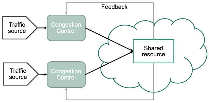
- Adjusts load introduced to shared resource in order to avoid overload situations
- Utilizes feedback information (implicit or explicit)
“Critical” Situations
Example 1
Router concurrently receives two packets from different input interfaces which are directed towards the same output interface. $\rightarrow$ Only one of these packets can be sent at a time.
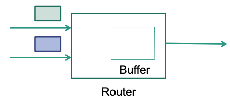
What to do with the other packet?
Buffer or
Drop
Example 2
Router has interfaces with different data rates
- Input interface has high data rate
- Output interface has low data rate
Two successive packets of a same or different senders arrive at input interface.
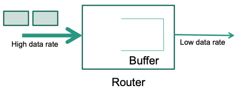
What to do with the second packet? The output interface is still busy sending the first packet while the second arrives.
- Buffer or
- Drop
Buffer
Routers need buffers (queues) to cope with temporary traffic bursts
Packets that can NOT be transmitted immediately are placed in the buffer
If buffer is filled up, packets need to be dropped 🤪
Buffers add latency
Typically implemented as FIFO queues
Router can only start sending a queued packet after all packets in front of it have been sent
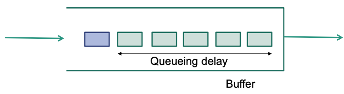
Five green packets introduce queueing delay for blue packet
End-to-end latency of a packet includes
- Propagation delay
- Transmission delay
- Queueing delay
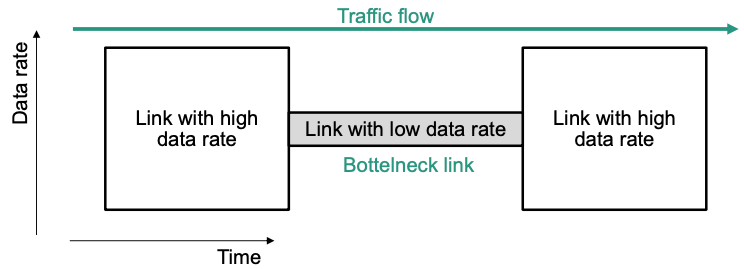
General Problem
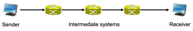
Sender wants to send data through the network to the receiver
On every network path, the link with the lowest available data rate limits the maximum data rate that can be achieved end-to-end
- This link is called bottleneck link
- The maximum data rate of a link is called link capacity
🔴 Problem: sender can send more data than bottleneck link can handle
Sender can overload bottleneck link! 🤪
$\rightarrow$ Sender has to adjust its sending rate
How to find the “optimal” sending rate?
Congestion Control vs. Flow Control
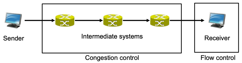
- Flow control
- Bottleneck is located at receiver side
- Receiver can not cope with desired data rate of sender
- Congestion control
- Bottleneck is located in the network
- Bottleneck link does not provide sufficient available data rate
- Leads to congested router / intermediate system
Congestion Collapse
Throughput vs. Goodput
Throughput: Amount of network layer data delivered in a time interval
- E.g., 1 Gbit/s
- Counts everything including retransmissions
$\rightarrow$ the aggregated amount of data that flows through the router/link
Goodput: „Application-level“ throughput
- Amount of application data delivered in a time interval
- Retransmissions at the transport layer do NOT count
- Packets dropped in transmission do NOT count
Observation
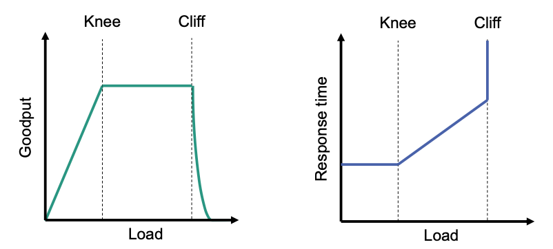
Load is small (below network capacity) $\rightarrow$ network keeps up with load
Load reaches network capacity (knee)
Goodput stops increasing, buffers build up, end-to-end latency increases
$\rightarrow$ Network is congested!
Load increases beyond cliff
- Packets start to be dropped, goodput drastically decreases $\rightarrow$ Congestion collapse
- Load refers to aggregated network layer traffic that is introduced by all active data streams. This includes TCP retransmissions.
- Network capacity refers to maximum load that network can handle.
How Could Congestion Collapse Happen?
Congestion due to
- Single TCP connection
- Exceeds available capacity at bottleneck link
- Prerequisite: flow control window is large enough
- Multiple TCP connections
- Aggregated load exceeds available capacity
- Single TCP connection has no knowledge about other TCP connections
Knee and Cliff
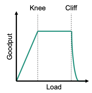
Keep traffic load around knee
- Good utilization of network capacity
- Low latencies
- Stable goodput
Prevent traffic from going over the cliff
- High latencies
- High packet losses
- Highly decreased goodput
Challenge of Congestion Control
- Challenge: Find “optimal” sending rate
- Usually, sender has NO global view of the network
- NO trivial answer
- Lots of algorithms for congestion control
Types of Congestion Control
Window-based Congestion Control
Congestion Control Window (𝐶𝑊𝑛𝑑)
- Determines maximum number of unacknowledged packets allowed per TCP connection
- Assumes that packets are acknowledged by receiver
- Basic window mechanism is similar to sliding window as applied for flow control purposes
- Adjusts sending rate of source to bottleneck capacity $\rightarrow$ self-clocking
Rate-based Congestion Control
Controls sending rate, no congestion control window
- Implemented by timers that determine inter packet intervals
- High precision required
- 🔴 Problem: NO comparable cut-off mechanism, such as missing acknowledgements
- Sender keeps sending even in case of congestion
- Needed in case no acknowledgements are used
- E.g., UDP
Implicit vs. Explicit Congestion Signals
Inplicit
- Without dedicated support of the network
- Implicit congestion signals
- Timeout of retransmission timer
- Receipt of duplicate acknowledgements
- Round-Trip Time (RTT) variation
Explicit
- Nodes inside the network indicate congestion
On the internet
- Usually NO support for explicit congestion signals
- Congestion control must work with implicit congestion signals only
End-to-end vs. Hop-by-hop
End-to-end
- Congestion control operates on an end system basis
- Nodes inside the network are NOT involved
Hop-by-hop
- Congestion control operates on a per hop basis
- Nodes inside the network are actively involved
Improved Versions of TCP
🎯 Goal
- Estimate available network capacity in order to avoid overload situations
- Provide feedback (congestion signal)
- Limit the traffic introduced into the network accordingly
- Apply congestion control
TCP Tahoe
TCP Recap
- Connection establishment
- 3 way handshake $\rightarrow$ Full duplex connection
- Connection termination
- Separately for each direction of transmission
- 4 way handshake
- Data transfer
- Byte-oriented sequence numbers
- Go-back-N
- Positive cumulative acknowledgements
- Timeout
- Flow control (sliding window)
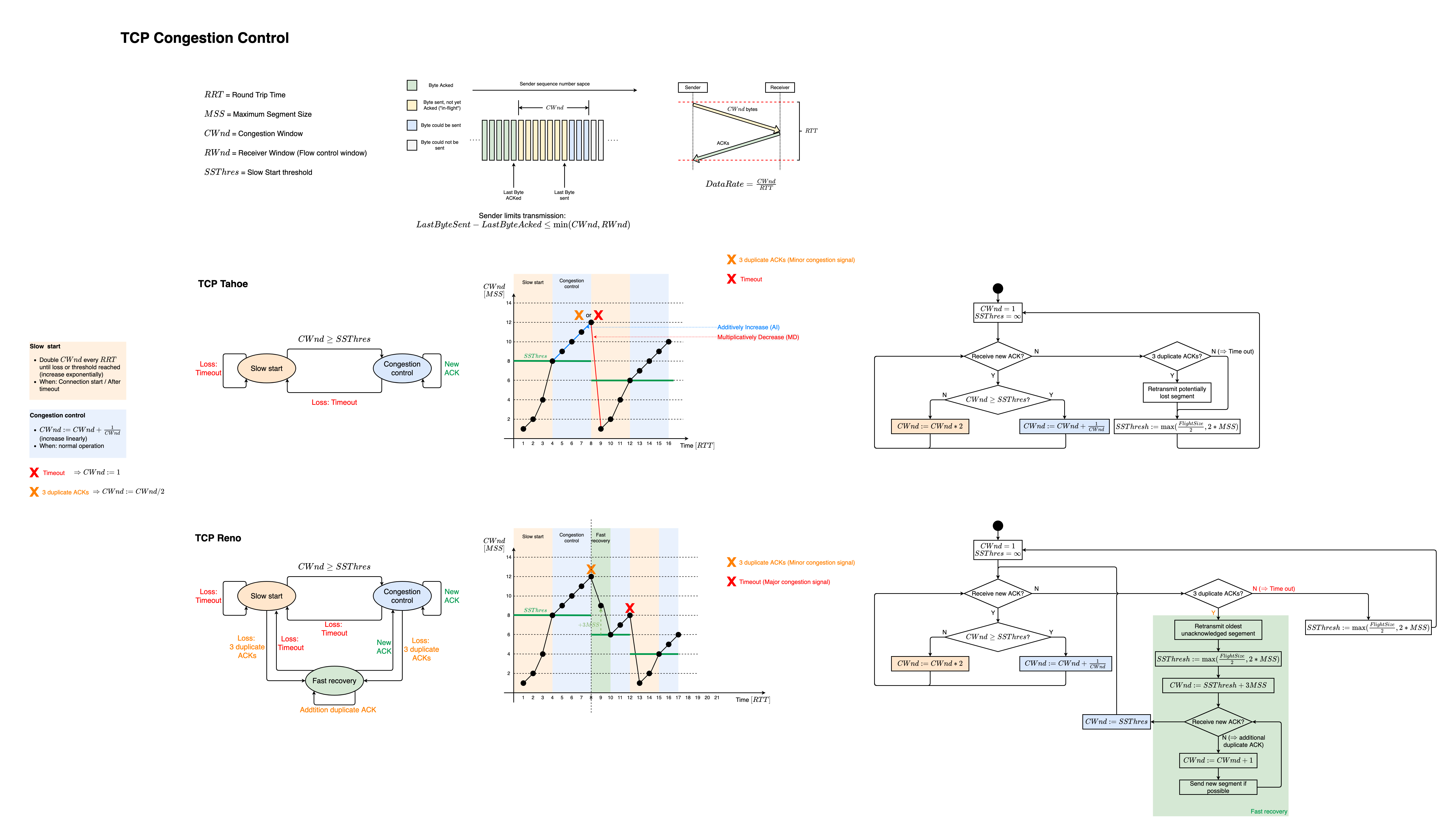
TCP Tahoe in a Nutshell
Mechanisms used for congestion control
- Slow start
- Timeout
- Congestion avoidance
- Fast retransmit
Congestion signal
- Retransmission timeout or
- Receipt of duplicate acknowledgements (𝑑𝑢𝑝𝑎𝑐𝑘)
$\rightarrow$ In case of congestion signal: slow start
The following must always be valid
$$ \text { LastByteSent }-\text { LastByteAcked } \leq \text { min\{CWnd, RcvWindow\} } $$- $\text{CWnd}$: Congestion Control Window
- $\text{RcvWindow}$: Flow Control Window
Variables
- $\text{CWnd}$: Convestion window
- $\text{SSThres}$: Slow Start Threshold
- Value of $\text{CWnd}$ at which TCP instance switches from slow start to congestion avoidance
Baisc approach: AIMD (additive increase, multiplicative decrease)
- Additive increase of $\text{CWnd}$ after receipt of an acknowledgement
- Multiplicative decrease of $\text{CWnd}$ if packet loss is assumed (congestion signal)
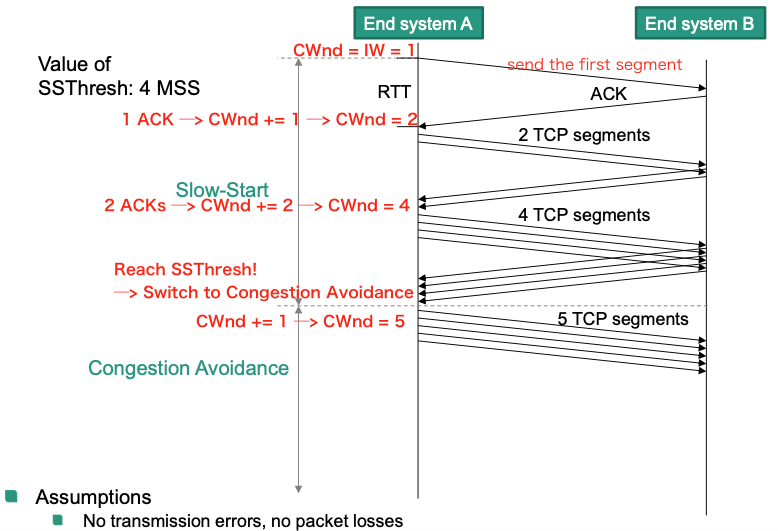
Initial values
- $\text{CWnd}=1 \text{ MSS}$
- $\text{MSS}$: Maximum Segment Size
- Since RFC 2581: Initial Window $\text{IW} \leq 2 \cdot \text{MSS}$ and $\text{CWnd}=\text{IW}$
- $\text{SSThres}$ initially set to “infinite”
- Number of duplicate ACKs (congestion signal): 3
- $\text{CWnd}=1 \text{ MSS}$
Algorithm
$\text{CWnd} < \text{SSThres}$ and ACKs are being received: slow start
- Exponential increase of congestion window
- Upon receipt of an ACK: $\text{CWnd } \text{+= } 1$
- Exponential increase of congestion window
$\text{CWnd} \geq \text{SSThres}$ and ACKs are being received: congestion avoidance
- Linear increase of congestion window
- Upon receipt of an ACK : $\text{CWnd } \text{+= } 1/\text{CWnd}$
- Linear increase of congestion window
Congestion signal: timeout or 3 duplicate acknowledgements: slow start
Congestion is assumed
Set
$$ \text { SSThresh }=\max (\text { FlightSize } / 2, 2 * M S S) $$- $\text { FlightSize }$: amount of data that has been sent but not yet acknowledged
- This amount is currently in transit
- Might also be limited due to flow control
- $\text { FlightSize }$: amount of data that has been sent but not yet acknowledged
Set $\text{CWnd}=1 \text{ MSS}$ or $\text{CWnd}=\text{IW}$
On 3 duplicate ACKs: retransmission of potentially lost TCP segment
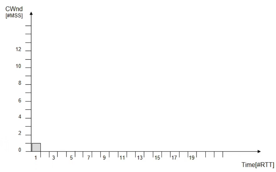
Example
Evolution of Congestion Window
Assumptions
- No transmission errors, no packet losses
- All TCP segments and acknowledgements are transmitted/received within single RTT
- Flight-size equals CWnd
- Congestion signal occurs during RTT
Initialize $\text{CWnd} = 1 \text{ MSS}$
The $\text{CWnd}$ grows in “slow start” mode. When $\text{CWnd} = 16$, a timeout error occurs.
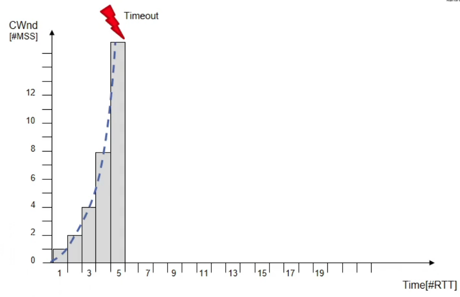
This is a congestion signal. So we go back to “slow start”
Set $\text { SSThresh }=\max (\text { FlightSize } / 2, 2 * M S S)$
In this case, $\text{FlightSize} = 16$.
So$\text { SSThresh }=\max (16 / 2, 2) \text{ MSS} = 8 \text{ MSS}$
Set $\text{CWnd}=1 \text{ MSS}$ or $\text{CWnd}=\text{IW}$
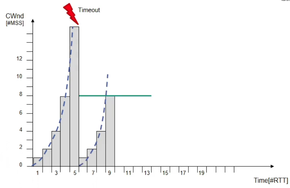
Now $\text{CWnd} \geq \text{SSThres}$ $\rightarrow$ Switch to “congestion avoidance”!
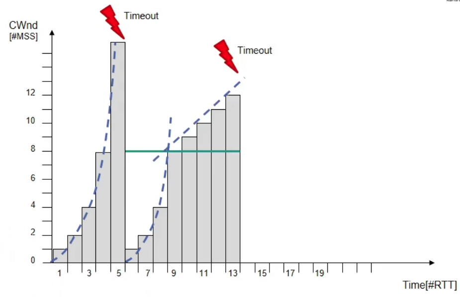
When $\text{CWnd} = 12$, a timeout error occurs.
We just perform the same handling as above.
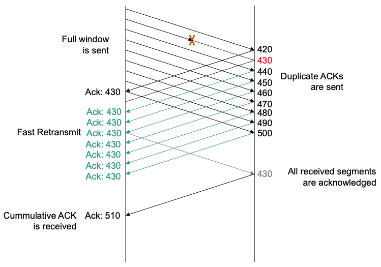
Fast Retransmit
Assume the following scenario
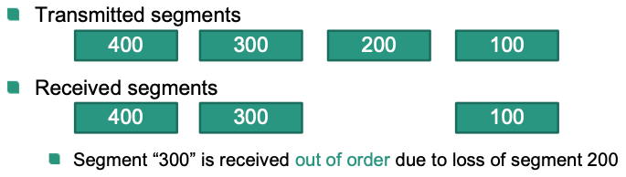
(Note: Not every segment that is received out of order indicates congestion. E.g., only one segment is dropped, otherwise data transfer is ok)
What would happen? Wait until retransmission timer expires, then retransmission
Waiting time is longer than a round trip time (RTT) $\rightarrow$ It will take a long time!🤪
Our goal is faster reaction
Retransmission after receipt of a pre-defined number of duplicate ACK
$\rightarrow$ Much faster than waiting for expiration of retransmission timer
Example: suppose pre-defined number of duplicate ACK is 3
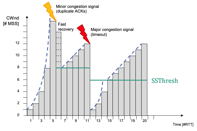
TCP Reno
Differentiation between
- Major congestion signal: Timeout of retransmission timer
- Minor congestion signal: Receipt of duplicate ACKs
In case of a major congestion signal
- Reset to slow start as in TCP Tahoe
In case of minor congestion signal
No reset to slow start
- Receipt of duplicate ACK implies successful delivery of new segments, i.e., packets have left the network
- New packets can also be injected in the network
In addition to the mechanisms of TCP Tahoe: fast recovery
- Controls sending of new segments until receipt of a non-duplicate ACK
Fast Recovery
- Starting condition: Receipt of a specified number of duplicate ACKs
- Usually set to 3 duplicate ACKs
- 💡 Idea: New segments should continue to be sent, even if packet loss is not yet recovered
- Self clocking continuous
- Reaction
- Reduce network load by halving the congestion window Retransmit first missing segment (fast retransmit)
- Consider continuous activity, i.e., further received segments while no new data is acknowledged
- Increase congestion window by number of duplicate ACKs (usually 3)
- Further increase after receipt of each additional duplicate ACK
- Receipt of new ACK (new data is acknowledged)
- Set congestion window to its value at the beginning of fast recovery
In Congestion Avoidance
- If timeout: slow start
- Set $\text { SSThresh }=\max (\text { FlightSize } / 2, 2 * M S S)$
- $\text{CWnd}=1$
- If 3 duplicate ACKs: fast recovery
- Retransmission of oldest unacknowledged segment (fast retransmit)
- Set $\text { SSThresh }=\max (\text { FlightSize } / 2, 2 * M S S)$
- Set $\text{CWnd} = \text{SSThresh} + 3\text{MSS}$
- Receipt of additional duplicate ACK
- $\text{CWnd } \text{+= } 1$
- Send new, i.e., not yet sent segments (if available)
- Receipt of a “new” ACK: congestion avoidance
- $\text{CWnd} = \text{SSThresh}$
Evolution of Congestion Window with TCP Reno
Analysis of Improvements
- After observing congestion collapses, the following mechanisms (among others) were introduced to the original TCP (RFC 793)
Slow-Start
Round-trip time variance estimation
Exponential retransmission timer backoff
Dynamic window sizing on congestion
More aggressive receiver acknowledgement policy
- 🎯 Goal: Enforce packet conservation in order to achieve network stability
Self Clocking
Recap: TCP uses window-based flow control
Basic assumption
- Complete flow control window in transit
- In TCP: receive window $𝑅𝑐𝑣𝑊𝑖𝑛𝑑𝑜𝑤$
- Bottleneck link with low data rate on the path to the receiver
- Complete flow control window in transit
Basic scenario

Conservation of Packets
🎯 Goal: get TCP connection in equilibrium
Full window of data in transit
“Conservative”: NO new segment is injected into the network before an old segment leaves the network
$\rightarrow$ A system with this property should be robust in the face of congestion
Three ways for packet conservation to fail
Slow Start
🎯 Goal: bring TCP connection into equilibrium
Connection has just started or
Restart after assumption of (major) congestion
🔴 Problem: get the „clock“ started (At the beginning of a connection there is no „clock“ available.)
💡 Basic idea (per TCP connection)
- Do not send complete receive window (flow control) immediately
- Gradually increase number of segments that can be sent without receiving an ACK
- Increase the amount of data that can be in transit (“in-flight”)
Approach
Apply congestion window, in addition to receive window
- Minimum of congestion and receive window can be sent
- Congestion Window: $𝐶𝑊𝑛𝑑$ $[𝑀𝑆𝑆]$
- Receive Window: $Rcv𝑊𝑖𝑛𝑑𝑜𝑤$ $[𝐵𝑦𝑡𝑒]$
- Minimum of congestion and receive window can be sent
New connection or congestion assumed
$\rightarrow$ Reset of congestion window: $𝐶𝑊𝑛𝑑 = 1$
Incoming ACK for sent (not retransmitted) segment
- Increase congestion window by one: $𝐶𝑊𝑛𝑑 = 𝐶𝑊𝑛𝑑 + 1$
$\rightarrow$ Leads to exponential growth of 𝐶𝑊𝑛𝑑
- Sending rate is at most twice as high as the bottleneck capacity!
Retransmission Timer
Assumption: Complete receive window in transit
Alternative 1: ACK received
- A segment was delivered and, thus, exited the network $\rightarrow$ conservation of packets is fulfilled
Alternative 2: retransmission timer expired
Segment is dropped in the network: conservation of packets is fulfilled
Segment is delayed but not dropped: conservation of packets NOT fulfilled
$\rightarrow$ Too short retransmission timeout causes connection to leave equilibrium
Good estimation of Round Trip Time (RTT) essential for a good timer value!
Value too small: unnecessary retransmissions
Value too large: slow reaction to packet losses
Estimation of Round Trip Time
Timer-based RTT measurement
- Timer resolution varies (up to 500 ms)
- Requirements regarding timer resolutions vary
SampleRTT
- Time interval between transmission of a segment and reception of corresponding acknowledgement
- Single measurement
- Retransmissions are ignored
EstimatedRTT
- Smoothed value across a number of measurements
- Observation: measured values can fluctuate heavily
Apply exponential weighted moving average (EWMA)
- Influence of each value becomes gradually less as it ages
- Unbiased estimator for average value
(Typical value for $\alpha$: 0.125)
Derive value for retransmission timeout (RTO)
$$ 𝑅𝑇𝑂 = \beta ∗ 𝐸𝑠𝑡𝑖𝑚𝑎𝑡𝑒𝑑𝑅𝑇𝑇 $$- Recommended value for $\beta$: 2
Estimation of Deviation
🎯 Goal: Avoid the observed occasional retransmissions
Observation: Variation of RTT can greatly increase in higher loaded networks
- Consequently, $EstimatedRTT$ requires higher “safety margin”
- Estimation error: difference between measured/sampled and estimated RTT
Computation
$$ \begin{array}{l} &Deviation =(1-\gamma) * Deviation+\gamma * \left|SampleRTT- EstimatedRTT \right| \\\\ &RTO =EstimatedRTT +\beta * Deviation \end{array} $$- Recommended values: $\alpha = 0.125, \beta = 4, \gamma = 0.25$
Multiple Retransmissions
How large should the time interval be between two subsequent retransmissions of the same segment?
Approach: Exponential backoff
After each new retransmission RTO doubles:
$$ 𝑅𝑇𝑂 = 2 ∗ 𝑅𝑇𝑂 $$- Maximal value should be applied. It should be $$ 60 seconds
To which segment does the received ACK belong – to the original segment or to the retransmission?
- Approach: Karn‘s Algorithm
- ACKs for retransmitted segments are not included into the calculation of $EstimatedRTT$ and $Deviation$
- Backoff is calculated as before
- Timeout value is set to the value calculated by backoff algorithm until an ACK to a non-retransmitted segment is received
- Then original algorithm is reactivated
- Approach: Karn‘s Algorithm
Congestion Avoidance
Consider multiple concurrent TCP connections
Assumption: TCP connection operates in equilibrium
Packet loss is with a high probability caused by a newly started TCP connection
- New connection requires resources on bottleneck router/link
$\rightarrow$ Load of already existing TCP connection(s) needs to be reduced
Basic components
Implicit congestion signals
- Retransmission timeout
- Duplicate acknowledgements
Strategy to adjust traffic load: AIMD
- Additively increase load if no congestion signal is experienced
On acknowledgement received: $𝐶𝑊𝑛𝑑 += 1/𝐶𝑊𝑛𝑑$
Multiplicatively decrease load in case a congestion signal was experienced
- On retransmission timeout
  $$
  CWnd = \gamma * CWnd, \quad 0< \gamma < 1
$$
- In TCP Tahoe: $\gamma = 1/2
Optimization Criteria
Basic Scenario
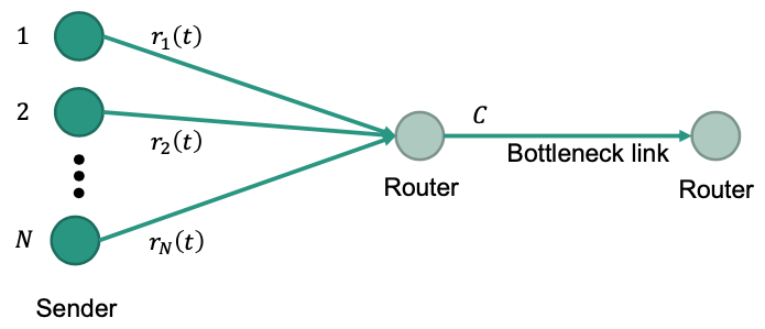
- $𝑁$ sender that use same bottleneck link
Data rate of sender $i$: $r\_i(t)$
Capacity of bottleneck link: $C$
- Bottleneck link: Link with lowest available data rate on the path to the receiver
Network-limited sender
- Assume that the sender always has data to send and data are sent as quickly as possible
- Sender can send a full window of data
- Congestion control limits the data rate of such a sender to the available capacity at the bottleneck link
Application-limited sender
- Data rate of the sender is limited by the application and not by the network
- Sender sends less data as allowed by the current window
Efficiency
- Closeness of the total load on the bottleneck link to its link capacity
- $\sum\_{j=1}^{N} r\_{i}(j)$ should be as close to 𝐶 as possible, i.e., close to the knee
- Overload and underload are not desirable
Fairness
All senders that share the bottleneck link get a fair allocation of the bottleneck link capacity
Examples
Jain ́s fairness index
Quantify „amount“ of unfairness
$$ F\left(r\_{i}, \ldots, r\_{N}\right)=\frac{\left(\sum r\_{i}\right)^{2}}{N\left(\sum r\_{i}^{2}\right)} $$Fairness index $\in [0, 1]$
- Totally fair allocation has fairness index of $1$ (i.e., all $r\_i$ are equal)
- Totally unfair allocation has fairness index of $1/N$ (i.e., one user gets entire capacity)
Max-min fairness
Situation
- Users share resource. Each user has an equal right to the resource
- But: some users intrinsically demand fewer resources than others (E.g., in case of application-limited senders)
Intuitive allocation of fair share
- Allocates users with a “small” demand what they want
- Equally distributes unused resources to “big” users
💡 Max-min fair allocation
Resources are allocated in order of increasing demand
No source gets a resource share larger than its demand
Sources with unsatisfied demands get an equal share of the resource
Implementation
- Senders $1, 2, ... 𝑁$ with demanded sending rates $s\_1, s\_2, ..., s\_N$
- Without loss of generality: $s\_1 \leq s\_2 \leq ...\leq s\_N$
- $C$: capacity
- Give $\frac{C}{N}$ to sender with smallest demand
- In case this is more than demanded, then $\frac{C}{N}− s\_1$ is still available to others
- $\frac{C}{N} − s\_1$ equally distributed to others $\Rightarrow$ each gets $ \frac{C}{N} + \frac{\frac{C}{N} - s\_1}{N- 1}$
- Senders $1, 2, ... 𝑁$ with demanded sending rates $s\_1, s\_2, ..., s\_N$
Example
Convergence
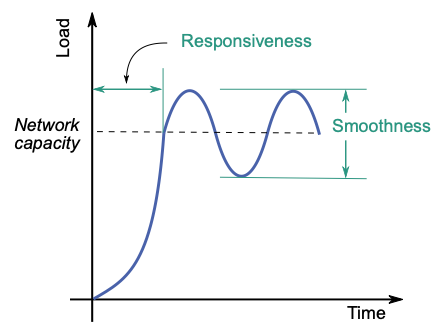
- Responsiveness: Speed with which $r\_i$ gets to equilibrium rate at knee after starting from any starting state
- May oscillate around goal (= network capacity)
- Smoothness: Size of oscillations around network capacity at steady state
(Smaller is better in both cases)
On Fairness
How to divide resources among TCP connections?
$\rightarrow$ Strive for fair allocation 💪
🎯 Goal: all TCP connections receive equal share of bottleneck resource
- the share should be non-zero
- equal share is not ideal for all applications 🤔
Example: $𝑁$ TCP connections share same bottleneck, Each TCP connection receives $(1/𝑁)$-th of bottleneck capacity
Observation
“Greedy” user: opens multiple TCP connections concurrently
Example
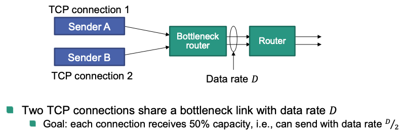
Link with capacity $𝐷$, two users, one connection per user
$\rightarrow$ Each user gets capacity $\frac{D}{2}$
Link with capacity $𝐷$, two users, user 1 with a single connection, user 2
with nine connections
$\rightarrow$ User 1 can use $\frac{1}{10}D$ , user 2 can use $\frac{9}{10}D$
“Greedy” receiver
- Can send several ACKs per received segment
- Can send ACKs faster than it receives segments
Additive Increase Multiplicative Decrease
General feedback control algorithm
Applied to congestion control
Additive increase of data rate until congestion
Multiplicative decrease of data rate in case of congestion signal
Converges to equal share of capacity at bottleneck link
AIMD: Fairness
- Network with two sources that share a bottleneck link with capacity $𝐶$
- 🎯 Goal: bring system close to optimal point $(\frac{𝐶}{2} , \frac{𝐶}{2})$
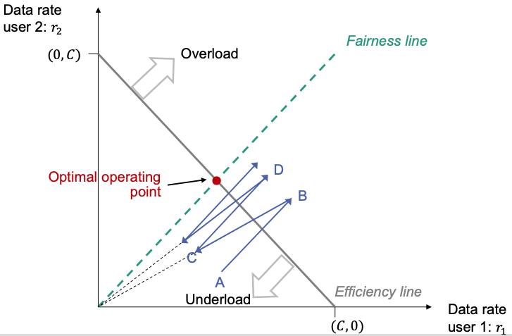
Efficiency line
- $r\_1 + r\_2 = C$ holds for all points on the line
- Points under the line means underloaded $\rightarrow$ Control decision: increase rate
- Points above the line means overloaded $\rightarrow$ Control decision: decrease rate
Fairness line
- All allocations with fair allocation, i.e. $r\_1 = r\_2$
- Multiplying with $𝑏$ does not change fair allocation: $br\_1 = br\_2$
Optimal operating point
- Intersection of efficiency line and fairness line: point $(\frac{𝐶}{2} , \frac{𝐶}{2})$
Optimality of AIMD
Additive increase
- Resource allocation of both users increased by $\alpha$
- In the graph: moving up along a 45-degree line
Multiplicative decrease
Move down along the line that connects to the origin
$\rightarrow$ Point of operation iteratively moves closer to optimal operating point 👏
Periodic Model
Performance metrics of interest
- Throughput How much data can be transferred in which time interval?
- Latency How high is the experienced delay?
- Completion time How long until the transfer of an object/file is finished?
Variables
- $X$: Sending rate measured in segments per time interval
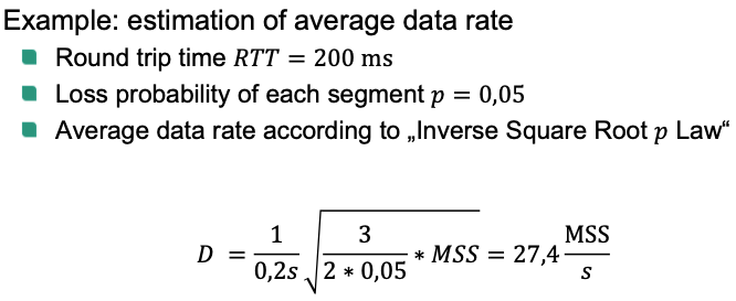
- $RTT$: Round trip time [seconds]
- $p$: Loss probability of a segment
- $MSS$: Maximum segment size [bit]
- $W$: Value of a congestion window [MSS]
- $D$: Data rate measured in bit per second [bit/s]
Periodic Model
Simple model – strong simplifications
🎯 Goals
Model long-term steady state behavior of TCP
Evaluate achievable throughput of a TCP connection under certain network conditions
Basic assumptions
- Network has constant loss probability $p$
- Observed TCP connection does not influence $p$
Further simplification: periodic losses
For an individual connection segment losses are equally spaced
$\rightarrow$ Link delivers $N = \frac{1}{p}$ segments followed by a segment loss
Additional simplifications / model assumptions
Slow start is ignored
Congestion window increases linearly (congestion avoidance)
RTT is constant
Losses are detected using duplicate ACKs (No timeouts)
Retransmissions are not modelled
- Go-Back-N is not modelled
Connection only limited by $CWnd$
- Flow control (receive window) is never a limiting factor
Always $MSS$ sized segments are sent
Under given assumptions we have the diagram:
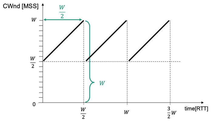
- Progress of CWnd: Perfect periodic saw tooth curve $$ \frac{W}{2}*MSS \leq CWnd \leq W * MSS $$ Note: Here $W$ is unitless.
Data rate when segment loss occurs?
$$ D = \frac{W * MSS}{RTT} $$How long until congestion window reaches 𝑊 again?
$$ \frac{W}{2} * RTT $$Average data rate of a TCP connection?
$$ D = \frac{0.75W * MSS}{RTT} $$
Step 1: Determine $W$ as a function of $p$
Minimal value of congestion window: $\frac{W}{2}$
Congestion window opens by one segment per RTT
- Duration of a period: $$ t = \frac{W}{2} \text{ round trip times } = \frac{W}{2}*RTT \text{ seconds } $$
Number of delivered segments within one period
Corresponds to the area under the saw tooth curve
$$ N=\left(\frac{W}{2}\right)^{2}+\frac{1}{2}\left(\frac{W}{2}\right)^{2}=\frac{3}{8} W^{2} $$According to the assumptions $N = \frac{1}{p}$
$\Rightarrow W = \sqrt{\frac{8}{3p}}$
Step 2: Determine data rate $D$ as a function of $p$
Average data rate
$$ D=\frac{N * M S S}{t} $$We have assumption $N = \frac{1}{p}$ and period duration is $\frac{W}{2}*RTT$ [s]
$$ \Rightarrow D=\frac{\frac{1}{p} * M S S}{R T T * \frac{W}{2}} $$In step 1 we have $W=\sqrt{\frac{8}{3 p}}$
$$ D=\frac{1}{R T T} \sqrt{\frac{3}{2 p}} * M S S $$This is called “Inverse Square-Root $𝑝$ Law”
Example
Active Queue Management (AQM)
Simple Queue Management
- Buffer in the router is full
- Next segment must be dropped $\rightarrow$ Tail drop
- TCP detects congestion and backs off
- 🔴 Problems
- Synchronization: Segments of several TCP connections are dropped (almost) at the same time
- Nearly full buffer cannot absorb short bursts
Active Queue Management
Basic approach
Detect arising congestion within the network
Give early feedback to senders
- Intentionally trigger implicit congestion signal: packet loss
- Alternative: Send explicit congestion notification (ECN)
Routers drop (or mark) segments, before queue completely filled up
- Randomization: random decision on which segment to be dropped
Observations at the receiver on layer 4 Typically only a single segment is missing
AQM algorithms
- Random Early Detection (RED)
- Newer algorithms: CoDel, FQ-CoDel, PIE …
Random Early Detection
Approach
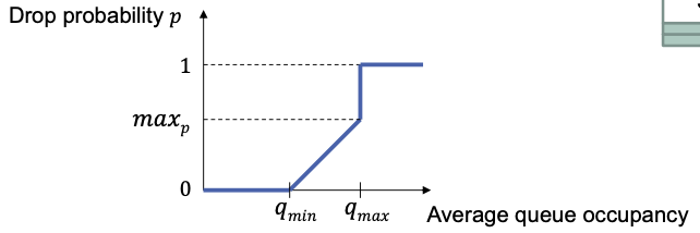
Average queue occupancy $< q\_{min}$
- No drop of segments ($𝑝 = 0$)
$q\_{min} \leq$ average queue occupancy $< q\_{max}$
- Probability of dropping an incoming packet is linearly increased with average queue occupancy
Average queue occupancy $ \geq q\_{max}$
- Drop all segments ($𝑝 = 1$)
Explicit Congestion Notification
🎯 Goal: Send explicit congestion signal, avoid unnecessary packet drops
Approach
Enable AQM to explicitly notify about congestion
AQM does not have to drop packets to create implicit congestion signal
How to notify?
- Mark IP datagram, but do not drop it
- Marked IP datagram is forwarded to receiver
How to react?
- Marked IP datagram is delivered to receiver instance of IP
- Information must be passed to corresponding receiver instance of TCP
- TCP sender must be notified