Ethernet
Aloha, Slotted Aloha
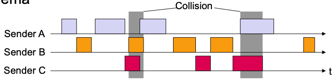
Aloha
First MAC protocol for packet-based wireless networks
Media access control (MAC)
- Time multiplex, variable, random access
- NO previous sensing of medium and no announcement of intended transmission
- Asynchronous access
🔴 Problem: Collision possible
Schema
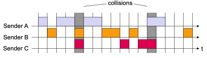
Slotted Aloha
Like Aloha, but
Uses time slots
- Synchronized access only at beginning of time slot
On average less collisions than with Aloha
Schema
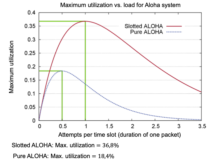
Evaluation
How well can the capacity of the medium be utilized?
Evaluation of Slotted Aloha
Assumptions
- Based on the design
- All systems start transmissions at beginning of time slot
- All systems work synchronized
- Simplifications
- All packets have same length and fit into one time slot
- If a collision arises, all systems notice it before end of the time slot
- All systems always want to send data
- Every system sends in each time slot with a probability of $𝑝$
- If a collision occurs
- Packet will be repeated with a probability of $𝑝$ in all following time slots until the transmission is successful
- All packets have same length and fit into one time slot
- Based on the design
There are $𝑁$ active systems in the network
- Probability that a system starts sending: $𝑝$
- Probability that $𝑁 − 1$ systems are not sending: $(1 - p)^{N-1}$
- Probability that a given system succeeds: $p(1 - p)^{N-1}$
- Probability for successful transmission of any one system: $Np(1 - p)^{N-1}$
Seeking for maximum utilization $U\_{max}$
Need $p^*$ s.t. $Np(1 - p)^{N-1}$ reaches its maximum
- Solution: $p^\* = \frac{1}{N}$
Therefore:
$$ \begin{array}{l} &N p^{\*}\left(1-p^{\*}\right)^{N-1}=\left(1-\frac{1}{N}\right)^{N-1}\\\\ &\displaystyle{\lim \_{N \rightarrow \infty}}\left(1-\frac{1}{N}\right)^{N-1}=\frac{1}{e}\\\\ &U\_{\max }=\frac{1}{e}=0.36 \end{array} $$
Evaluation of Aloha
Simplifying assumptions
- All packets have same length
- Immediate notification about collisions
- On collision: Packet will be repeated immediately with probability $𝑝$
- On successful transmission
- Wait for transmission time of packet
- Then: continue sending with probability $𝑝$ and continue waiting with probability $1 − 𝑝$
Observation: Collision occurs
a) if previous packet from other system has not been send completely, or
b) if other system starts sending before ongoing transmission is finished
There are $𝑁$ active systems in the network
- Probability that a system starts sending: $𝑝$
- Probability for (a) and (b): $(1 - p)^{N-1}$
- Probability for successful transmission of any one system: $Np(1 - p)^{2(N-1)}$
Further observations as for Slotted Aloha
$$ \begin{array}{l} \displaystyle{\lim\_{N \rightarrow \infty}} \frac{N}{2 N-1}\left(1-\frac{1}{2 N-1}\right)^{2(N-1)}=\frac{1}{2 e} \\\\ \Rightarrow U_{\max }=\frac{1}{2 e}=0.18 \end{array} $$
Comparison of Utilization Between Aloha and Slotted Aloha
CSMA-based Approaches
CSMA = Carrier Sense Multiple Access
- CSMA/CD
- CD = Collision Detection (“Listen before talk, listen while talk“)
- Sending system can detect collisions by listening
- Usage example: Ethernet
- CSMA/CA
- CA = Collision Avoidance
- Sending system assumes collisions when acknowledgement is missing
- MAC-layer acknowledgements, stop-and-wait
- Usage example: WLAN
Ethernet Variants
| Ethernet variants | Data rate | Topology | Medium access | Evaluation | Layers | Flow control |
|---|---|---|---|---|---|---|
| Original | 10 Mbit/s | bus | CSMA/CD | Utilization | 1 and 2a | |
| Fast Ethernet | 100 Mbit/s | star | CSMA/CD | Implicit / Explicit | ||
| Gigabit Ethernet | 1 Gbit/s | star | Carrier extension, frame bursting | |||
The Original
Standardized as IEEE 802.3
Medium access control
Time multiplex, variable, random access
Asynchronous access
Uses CSMA/CD
Collisions detection through listening
Exponential backoff
1-persistent
Network topology
- Originally: Bus topology
Data rate
- Originally: 10 Mbit/s
Wire based
- Originally: Coaxial cable
Standard consists of
Layer 1 and
Layer 2a (MAC-Protocol)
CSMA/CD-based approach
Check medium
- Considered free if no activity is detected for 96 bit times
- 96 bit times = Inter Frame Space (IFS)
- Considered free if no activity is detected for 96 bit times
Sending: 1-persistent
1-persistent
1-persistent CSMA is an aggressive transmission algorithm. When the transmitting node is ready to transmit, it senses the transmission medium for idle or busy.
- If idle, then it transmits immediately.
- If busy, then it senses the transmission medium continuously until it becomes idle, then transmits the message (a frame) unconditionally (i.e. with probability=1).
- In case of a collision, the sender waits for a random period of time and attempts the same procedure again.
1-persistent CSMA is used in CSMA/CD systems including Ethernet.
Collision detection by sender
- Abort sending
- Send jamming signal (length of 48 bit, format
1010...) - Ensure collision detection: Minimum length of frame
Exponential backoff for repeated transmissions
Collision Detection
Collision detection by sender
Detection must happen before transmission is finished
$\rightarrow$ We need Minimum duration for sending
Doubled maximum propagation delay $t\_a$ of the medium
$\rightarrow$ Minimum length of a 802.3-MAC frame required
In case of shorter frames
- No reliable collision detection 🤪
- No CSMA/CD, only CSMA 🤪
How to enforce minimum frame length?
- Implemented transparently for the application
- I.e., application can transmit small portions of data if desired
- Frame is extended by padding field (PAD)
- Implemented transparently for the application
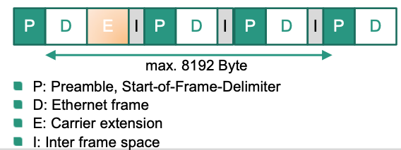
Ethernet Frame
Structure
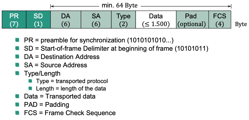
Between two frames: IFS
Evaluation Ethernet: Utilization
🎯 Goal: Derive upper bound of utilization $U\_{max}$
Assumption
Perfect protocol
- No transmission errors, no overhead, no processing time, …
Achieved throughput
$$ r\_{e}=\frac{X}{t\_{s}+t\_{a}}=\frac{X}{X / r+d / v} $$- $r\_e$: effective data rate
- $X$: #bits to transmit
- $t\_a$: propagation delay
- $t\_s$: transmission delay
- $r$: data rate
- $d$: medium distance
- $v$: transmission speed
Parameter $𝑎$ often used for performance evaluation
$$ a= \frac{\text{propagation delay}}{\text{transmission delay}} = \frac{t\_{a}}{t\_{s}}=\frac{d / v}{X / r}=\frac{r d}{X v} $$Utilization under optimal circumstances
$$ U\_{\max }=\frac{r\_{e}}{r}=\frac{1}{1+a} $$Local network with $𝑁$ active systems
- Each system can always send a frame
- System sends frames with probability $𝑝$
Maximum normalized propagation delay of $𝑎$
- I.e., transmission time $t\_s$ of each frame is normalized to 1
Time is logically partitioned in time slots
- Length is doubled end-to-end propagation delay (i.e., $2a$)
Observations
Two types of time intervals
Transmission intervals: $\frac{1}{2a}$ time slots
- Transmission time $t\_s$ is normalized to 1
- Length of each time slot is $2a$
$\Rightarrow$ We need $\frac{1}{2a}$ time slots
Collision intervals: collisions or no transmissions
Evaluation
$$ \lim \_{N \rightarrow \infty} U\_{\max }=\frac{1}{1+3.44 a} $$Details
Average length $l\_k$ of a collision interval (measured in time slots)
Probability $A$ that exactly one system is sending:
$$ A = Np(1 - p)^{N-1} $$Function has maximum at $p^\* = \frac{1}{N} \Rightarrow A^\* = (1 - \frac{1}{N})^{N-1}$
Probability that in $i$ following time slots a collision or no transmission occurs,
followed by a time slot with transmission
$$ \left(1-A^{\*}\right)^{i} A^{\*} $$Average length $l\_k$:
$$ E\left[l\_{k}\right]=\sum\_{i=1}^{\infty} i\left(1-A^{\*}\right)^{i} A^{\*} \to \frac{1-A^\*}{A\*} $$
Therefore
$$ U\_{\max }=\frac{\text { Transmission interval }}{\text { Transmission interval }+\text { Collision interval }} = \frac{1 /(2 a)}{1 /(2 a)+\left(1-A^{\*}\right) / A^{\*}}=\frac{1}{1+2 a\left(1-A^{\*}\right) / A^{\*}} $$For increasing number $N$ of systems
$$ \lim \_{N \rightarrow \infty} A^{\*}=\lim \_{N \rightarrow \infty}\left(1-\frac{1}{N}\right)^{N-1}=1 / e $$ $$ \Rightarrow \lim \_{N \rightarrow \infty} U\_{\max }=\frac{1}{1+3.44 a} $$
Fast Ethernet
- Standardization: 1995 standardized as IEEE 802.3u (100Base-TX)
- Important features
- Data rate: 100 Mbit/s
- Switchable between 10 Mbit/s and 100 Mbit/s
- Automatic negotiation
- Network topology: Star
- Medium access control
- CSMA/CD (for half duplex links)
- Preserve Ethernet frame format
- Modified encoding
- Data rate: 100 Mbit/s
Ethernet Flow Control
- Goal: Avoid packet losses due to buffer overflow
- Approach: Reduce traffic transmitted to the switch
- Apply flow control at layer 2
- Half-duplex links (shared LAN)
- Implicit flow control
- Backpressure: prevent potential transmitter from actually sending traffic
- Full-duplex links
- Explicit flow control
- Half-duplex links (shared LAN)
Implicit Flow Control
Half-duplex links
Two backpressure methods
- Enforce collision
- Pretend medium is busy
Explicit Flow Control
Full duplex link
Pause function
Receiver transmits PAUSE frame in case of an overload situation
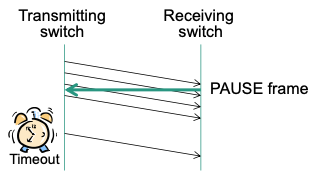
Sender stops transmitting data frames when receiving a PAUSE frame
Implicit continuation after pause time given in PAUSE frame (multiple of time for sending 512 bit)
Explicit continuation when receiving PAUSE frame with time=0
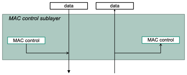
PAUSE function is part of the sublayer MAC control (extension of MAC layer)
MAC Control sublayer
Handling of frames
- MAC control frames terminate on the MAC control sublayer or are generated by it
- All other frames are passed from/to higher layers
MAC Control Frame

Type = 0x8808
MCC: MAC Control Opcode
- Code for selected control function
- 0x0001: PAUSE frame
MAC Control Parameters: Unused part filled with zeros at the end
Gigabit Ethernet
Important characteristics
- Data rate: 1 Gbit/s
- Network topology: Star
- Medium access control
- CSMA/CD (for half-duplex links)
- Preserve Ethernet frame format
New concepts
- Modify medium access control: Carrier extension
- Optional possibilities for improved throughput: Frame bursting
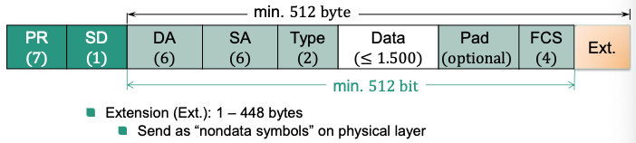
Carrier Extension
Goal: Ensure collision detection
Approach: Increase transmission delay without modifying Ethernet frame structure
Basic enhancements
Length of time slot ≠ minimum length of frame
- Minimum frame length: 512 bit
- New length of time slot: 512 byte
Frame with carrier extension
Frame Bursting
Goal: Efficient transmission of short frames
Approach: Systems are permitted to send burst of frames directly following each other
- First frame with extension, if required
- Following frames directly back-to-back (no extension)
Schema
Summary
- Today ́s Ethernet is very different from the original version developed by Metcalf and Boggs
- One constant has remained: The Ethernet frame format
Spanning Tree
Bridges
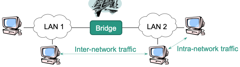
🎯 Goal: Connect local area networks (LANs) on layer 2
Properties
- Filter function: Detaches intra-network traffic in one LAN from inter-network-traffic to other LANs
Schema
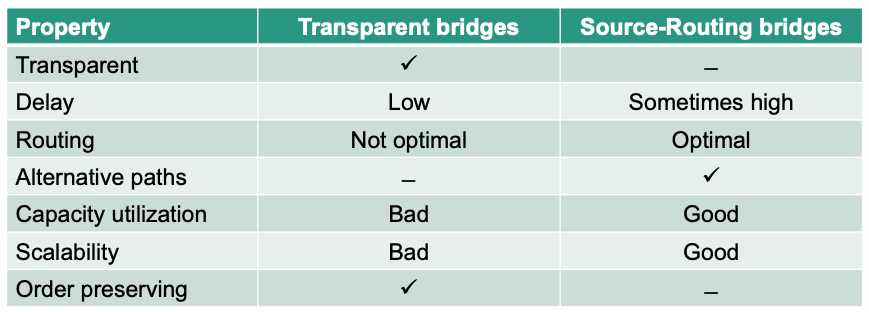
Types
Source-Routing bridges
- End systems add forwarding information in send packets
Bridges forward the packets based on this information
Sending packets is NOT transparent for the end system – it has to know the path
- Technically easy but not often used in practice 🤪
- End systems add forwarding information in send packets
Transparent bridges
Local forwarding decisions in each bridge
- Forwarding information normally stored in a table (forwarding table)
- Static entries as well as dynamically learned entries
End system is NOT involved in forwarding decisions
$\rightarrow$ Existence of bridges is transparent to end systems
Often used in practice (e.g., switches)
Comparison
Transparent Bridges resp. Switches
Important features
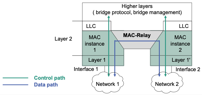
For each network interface exists an own layer 1 and MAC instance
Data path: Through MAC relay (implements forwarding on layer 2)
Control path
- E.g., bridge protocol, bridge management
- Logical Link Control (LLC) instances are involved
Basic Tasks
Establishing a loop-free topology
- s.t. Packets must not loop endlessly in the network
$\rightarrow$ Spanning-tree algorithm
Forwarding of packets
Learning the “location” of end systems
- Creation of the forwarding table
Filtering resp. forwarding of packets
- Based on the information of the forwarding table
Spanning-Tree Algorithm
Task
Organize bridges in a tree topology (NO loops!)
- Nodes: bridges and local networks
- Edges: connections between interfaces and local networks
Not all bridges have to be part of the tree topology
- Resources might not be used optimally
Forwarding of packets (Only possible along the tree)
Bridge protocol implements the Spanning-Tree algorithm
Requirements for using the bridge protocol
Group address to address all bridges in the network
Unique bridge identifier per bridge in the network
Unique interface identifier per interface in each bridge
Path costs for all interfaces of a bridge have to be known
BPDUs
Bridges send special packets: Bridge Protocol Data Units (BPDUs)
BPDU contains (among others)
Identifier of the sending bridge
Identifier of the bridge that is assumed as root bridge
Path cost from sending bridge to root bridge
Basic Steps
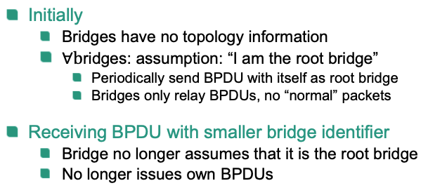
Determine root bridge
- Initially
- Bridges have no topology information
- All bridges: assumption: “I am the root bridge”
- Periodically send BPDU with itself as root bridge
- Bridges only relay BPDUs, no “normal” packets
- Receiving BPDU with smaller bridge identifier
- Bridge no longer assumes that it is the root bridge
- No longer issues own BPDUs
- When receiving BPDU possibly update of the configuration
- BPDU contains root bridge with smaller identifier
- BPDU with same root bridge identifier but cheaper path to root bridge
- Bridge notices that it is not the designated bridge $\rightarrow$ No longer forwards BPDUs
- Initially
Determine root interfaces for each bridge
- Calculate the path costs to the root bridge (Sum over costs of all interfaces on path to the root bridge)
- Select interface with the lowest costs
Determine designated bridge for each LAN (loop free!)
LAN can have multiple bridges
Select bridge with lowest costs on root interface
Responsible for forwarding of packets
Other bridges in the LAN will be deactivated
Stable Phase
- Root bridge periodically issues BPDUs
- Only “active” bridges forward BPDUs
- No more BPDUs are received
- Bridge again assumes that it is the root bridge
- Algorithm re-starts
- After stabilization packets are forwarded over the respective ports
- Based on the entries in the forwarding table
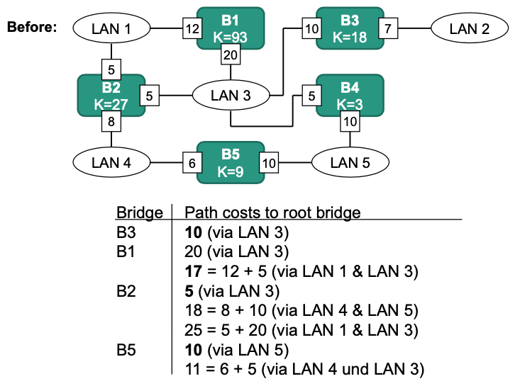
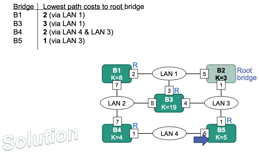
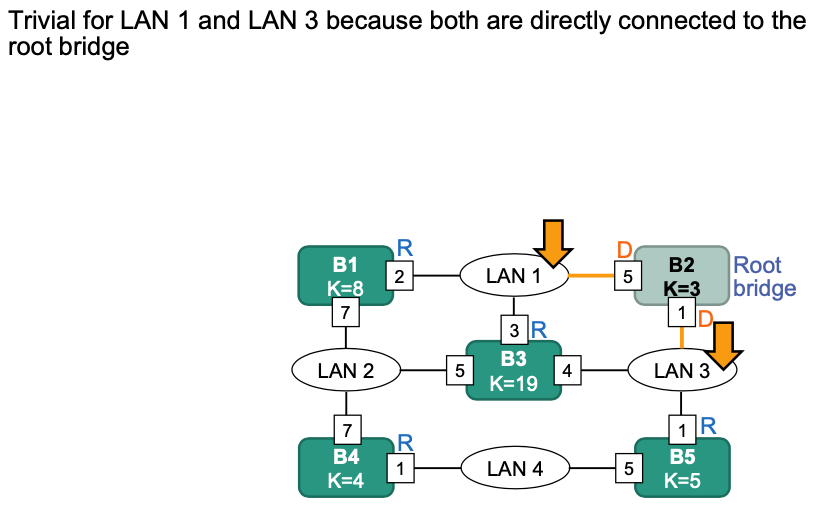
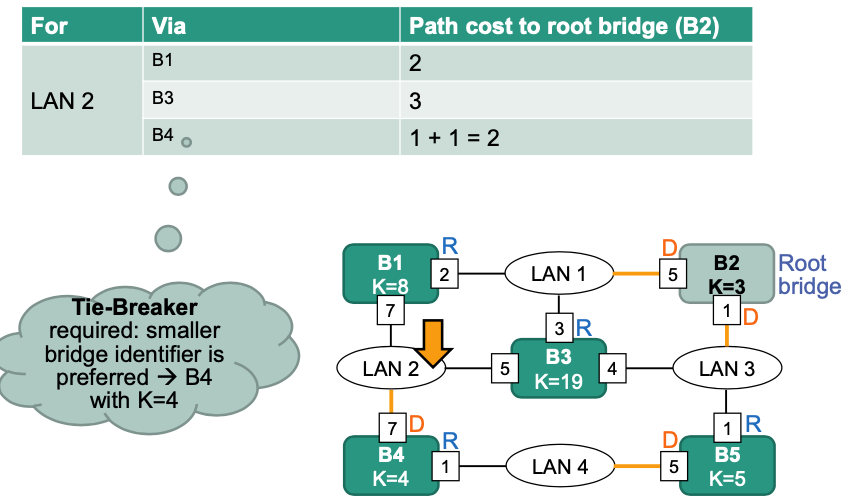
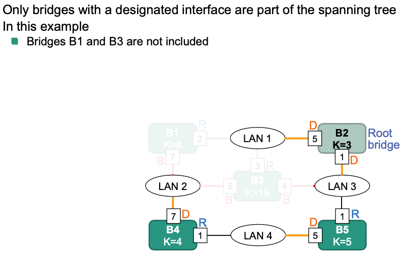
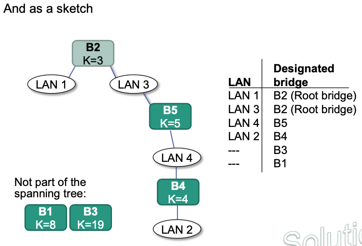
Example 1
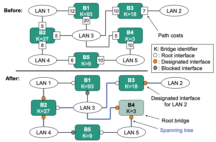
Calculate path costs to root bridge
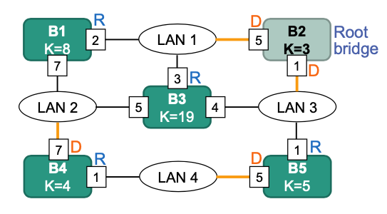
Determine designated bridges
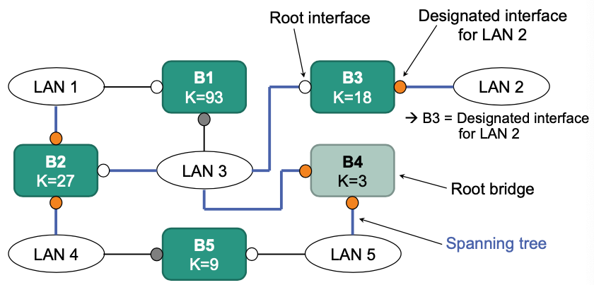
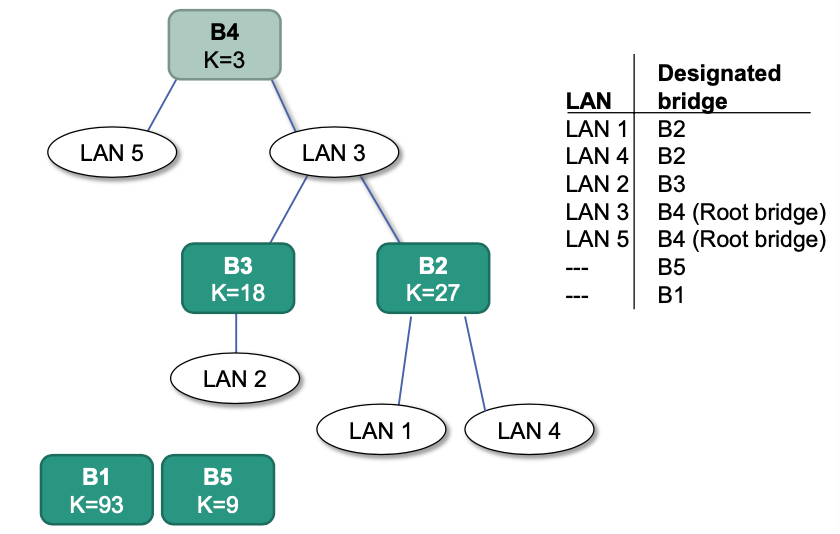
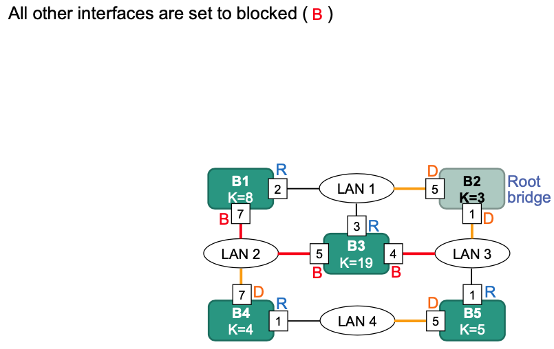
The resulting spanning tree:
Example 2
HW15
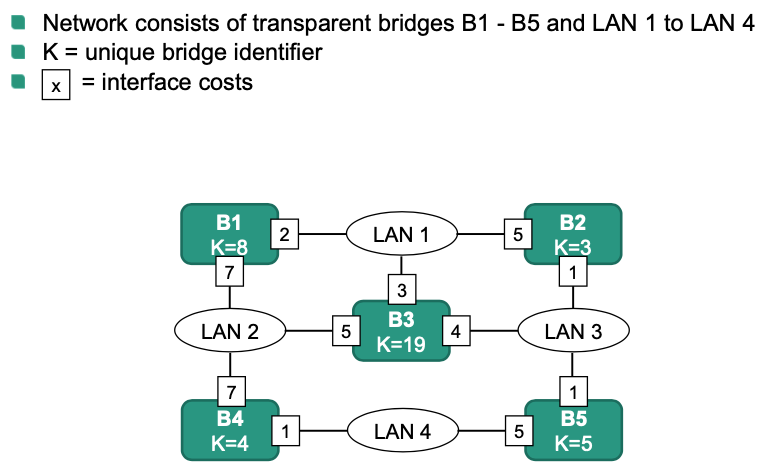
Solution:
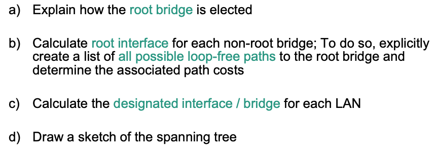
a)
b) Note: Root interface is for non-root bridge
c) When calculating designated interface, start from LAN and consider the shortest path
d)
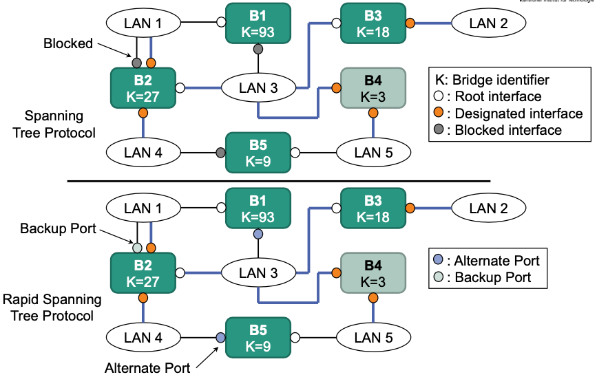
Rapid Spanning Tree Protocol (RSTP)
Overview of some relevant changes
- New port states
- Alternate Port: best alternative path to root bridge
- Backup Port: alternative path to a network that already has a connection
- Bridge has two ports which connect to the same network
- Sending BPDUs
- are additionally used as “keep-alive” messages
- Every bridge sends periodic BPDUs (Hello-Timer = 2s)
To the next hierarchy level in the tree
Failure of a neighbor: no BPDU for 3 times
- New port states
Example