Logistic Regression in NLP

Logistic Regression (in NLP)

In natural language processing, logistic regression is the base-line supervised machine learning algorithm for classification, and also has a very close relationship with neural networks.

Generative and Discriminative Classifier

The most important difference between naive Bayes and logistic regression is that

• logistic regression is a discriminative classifier while
• naive Bayes is a generative classifier.

Consider a visual metaphor: imagine we’re trying to distinguish dog images from cat images.

• Generative model
• Try to understand what dogs look like and what cats look like
• You might literally ask such a model to ‘generate’, i.e. draw, a dog
• Given a test image, the system then asks whether it’s the cat model or the dog model that better fits (is less surprised by) the image, and chooses that as its label.
• disciminative model
  • only trying to learn to distinguish the classes
  • So maybe all the dogs in the training data are wearing collars and the cats aren’t. If that one feature neatly separates the classes, the model is satisfied. If you ask such a model what it knows about cats all it can say is that they don’t wear collars.

More formally, recall that the naive Bayes assigns a class $c$ to a document $d$ NOT by directly computing $p(c|d)$ but by computing a likelihood and a prior

$$ \hat{c}=\underset{c \in C}{\operatorname{argmax}} \overbrace{P(d | c)}^{\text { likelihood prior }} \overbrace{P(c)}^{\text { prior }} $$

• Generative model (like naive Bayes)

  • Makes use of the likelihood term
    • Expresses how to generate the features of a document if we knew it was of class $c$

• Discriminative model

  • attempts to directly compute $P(c|d)$
  • It will learn to assign a high weight to document features that directly improve its ability to discriminate between possible classes, even if it couldn’t generate an example of one of the classes.

Components of a probabilistic machine learning classifier

• Training corpus of $M$ input/output pairs $(x^{(i)}, y^{(i)})$

• A feature representation of the input

  • For each input observation $x^{(i)}$, this will be a vector of features $[x_1, x_2, \dots, x_n]$
    • $x_{i}^{(j)}$: feature $i$ for input $x^{(j)}$

• A classification function that computes $\hat{y}$, the estimated class, via $p(y|x)$

• An objective function for learning, usually involving minimizing error on

  training examples

• An algorithm for optimizing the objective function.

Logistic regression has two phases:

• training: we train the system (specifically the weights $w$ and $b$) using stochastic gradient descent and the cross-entropy loss.

• test: Given a test example $x$ we compute $p(y|x)$ and return the higher probability label $y=1$ or $y=0$.

Classification: the sigmoid

Consider a single input observation $x = [x_1, x_2, \dots, x_n]$

The classifier output $y$ can be

• $1$: the observation is a member of the class
• $0$: the observation is NOT a member of the class

We want to know the probability $P(y=1|x)$ that this observation is a member of the class.

E.g.:

• The decision is “positive sentiment” versus “negative sentiment”
• the features represent counts of words in a document
• $P(y=1|x)$ is the probability that the document has positive sentiment, while and $P(y=0|x)$ is the probability that the document has negative sentiment.

Logistic regression solves this task by learning, from a training set, a vector of weights and a bias term.

• Each weight $w_i$ is a real number, and is associated with one of the input features $x_i$. The weight represents how important that input feature is to the classification decision, can be

  • positive (meaning the feature is associated with the class)
  • negative (meaning the feature is NOT associated with the class).

  E.g.: we might expect in a sentiment task the word awesome to have a high positive weight, and abysmal to have a very negative weight.

• Bias term $b$, also called the intercept, is another real number that’s added to the weighted inputs.

To make a decision on a test instance, the resulting single number $z$ expresses the weighted sum of the evidence for the class:

$$ \begin{array}{ll} z &=\left(\sum_{i=1}^{n} w_{i} x_{i}\right)+b \\ & = w \cdot x + b \\ & \in (-\infty, \infty) \end{array} $$

(Note that $z$ is NOT a legal probability, since $z \notin [0, 1]$)

To create a probability, we’ll pass $z$ through the sigmoid function (also called logistic function):

$$ y=\sigma(z)=\frac{1}{1+e^{-z}} $$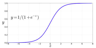

👍 Advantages of sigmoid:

• It takes a real-valued number and maps it into the range [0,1] (which is just what we want for a probability)
• It is nearly linear around 0 but has a sharp slope toward the ends, it tends to squash outlier values toward 0 or 1.
• Differentiable $\Rightarrow$ handy for learning

To make it a probability, we just need to make sure that the two cases, $P(y=1)$ and $P(y=0)$, sum to 1:

$$ \begin{aligned} P(y=1) &=\sigma(w \cdot x+b) \\ &=\frac{1}{1+e^{-(w \cdot x+b)}} \\ P(y=0) &=1-\sigma(w \cdot x+b) \\ &=1-\frac{1}{1+e^{-(w \cdot x+b)}} \\ &=\frac{e^{-(w \cdot x+b)}}{1+e^{-(w \cdot x+b)}} \end{aligned} $$

Now we have an algorithm that given an instance $x$ computes the probability $P(y=1|x)$. For a test instance $x$, we say yes if the probability is $P(y=1|x)$ more than 0.5, and no otherwise. We call 0.5 the decision boundary:

$$ \text{predict class}=\left\{\begin{array}{ll} 1 & \text { if } P(y=1 | x)>0.5 \\ 0 & \text { otherwise } \end{array}\right. $$

Example: sentiment classification

Suppose we are doing binary sentiment classification on movie review text, and we would like to know whether to assign the sentiment class + or − to a review document $doc$.

We’ll represent each input observation by the 6 features $x_1,...,x_6$ of the input shown in the following table

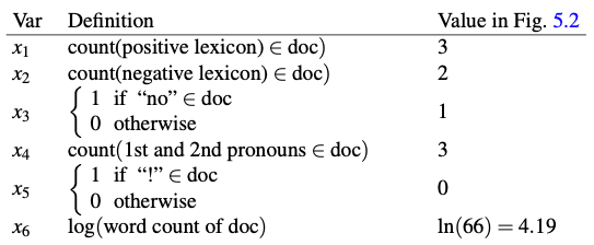
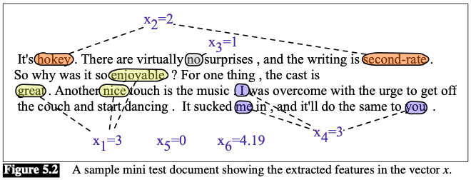
Assume that for the moment that we’ve already learned a real-valued weight for each of these features, and that the 6 weights corresponding to the 6 features are $w= [2.5,−5.0,−1.2,0.5,2.0,0.7]$, while $b = 0.1$.

• The weight $w_1$, for example indicates how important a feature the number of positive lexicon words (great, nice, enjoyable, etc.) is to a positive sentiment decision, while $w_2$tells us the importance of negative lexicon words. Note that $w_1 = 2.5$ is positive, while $w_2 = −5.0$, meaning that negative words are negatively associated with a positive sentiment decision, and are about twice as important as positive words.

Given these 6 features and the input review $x$, $P(+|x)$ and $P(-|x)$ can be computed:

$$ \begin{aligned} p(+| x)=P(Y=1 | x) &=\sigma(w \cdot x+b) \\ &=\sigma([2.5,-5.0,-1.2,0.5,2.0,0.7] \cdot[3,2,1,3,0,4.19]+0.1) \\ &=\sigma(0.833) \\ &=0.70 \\ p(-| x)=P(Y=0 | x) &=1-\sigma(w \cdot x+b) \\ &=0.30 \end{aligned} $$

$0.70 > 0.50 \Rightarrow$ This sentiment is positive ($+$).

Learning in Logistic Regression

Logistic regression is an instance of supervised classification in which we know the correct label $y$ (either 0 or 1) for each observation $x$.

The system produces/predicts $\hat{y}$, the estimate for the true $y$. We want to learn parameters ($w$ and $b$) that make $\hat{y}$ for each training observation as close as possible to the true $y$. 💪

This requires two components:

• loss function: also called cost function, a metric measures the distance between the system output and the gold output
  • The loss function that is commonly used for logistic regression and also for neural networks is cross-entropy loss
• Optimization algorithm for iteratively updating the weights so as to minimize this loss function
  • Standard algorithm: gradient descent

The Cross-Entropy Loss Function

We need a loss function that expresses, for an observation $x$, how close the classifier output ($\hat{y}=\sigma(w \cdot x+b)$) is to the correct output ($y$, which is $0$ or $1$):

$$ L(\hat{y}, y)= \text{How much } \hat{y} \text{ differs from the true } y $$

This loss function should prefer the correct class labels of the training examples to be more likely.

👆 This is called conditional maximum likelihood estimation: we choose the parameters $w, b$ that maximize the log probability of the true $y$ labels in the training data given the observations $x$. The resulting loss function is the negative log likelihood loss, generally called the cross-entropy loss.

Derivation

Task: for a single observation $x$, learn weights that maximize $p(y|x)$, the probability of the correct label

There’re only two discretions outcomes ($1$ or $0$)

$\Rightarrow$ This is a Bernoulli distribution. The probability $p(y|x)$ for one observation can be expressed as:

$$ p(y | x)=\hat{y}^{y}(1-\hat{y})^{1-y} $$

• $y=1, p(y|x)=\hat{y}$
• $y=0, p(y|x)=1-\hat{y}$

Now we take the log of both sides. This will turn out to be handy mathematically, and doesn’t hurt us (whatever values maximize a probability will also maximize the log of the probability):

$$ \begin{aligned} \log p(y | x) &=\log \left[\hat{y}^{y}(1-\hat{y})^{1-y}\right] \\ &=y \log \hat{y}+(1-y) \log (1-\hat{y}) \end{aligned} $$

👆 This is the log likelihood that should be maximized.

In order to turn this into loss function (something that we need to minimize), we’ll just flip the sign. The result is the cross-entropy loss:

$$ L_{C E}(\hat{y}, y)=-\log p(y | x)=-[y \log \hat{y}+(1-y) \log (1-\hat{y})] $$

Recall that $\hat{y}=\sigma(w \cdot x+b)$:

$$ L_{C E}(w, b)=-[y \log \sigma(w \cdot x+b)+(1-y) \log (1-\sigma(w \cdot x+b))] $$

Example

Let’s see if this loss function does the right thing for example above.

We want the loss to be

• smaller if the model’s estimate is close to correct, and

• bigger if the model is confused.

Let’s suppose the correct gold label for the sentiment example above is positive, i.e.: $y=1$.

• In this case our model is doing well 👏, since it gave the example a a higher probability of being positive ($0.70$) than negative ($0.30$).

  If we plug $\sigma(w \cdot x+b)=0.70$ and $y=1$ into the cross-entropy loss, we get

$$ \begin{aligned} L_{C E}(w, b) &=-[y \log \sigma(w \cdot x+b)+(1-y) \log (1-\sigma(w \cdot x+b))] \\ &=-[\log \sigma(w \cdot x+b)] \\ &=-\log (0.70) \\ &=0.36 \end{aligned} $$

By contrast, let’s pretend instead that the example was negative, i.e.: $y=0$.

• In this case our model is confused 🤪, and we’d want the loss to be higher.

  If we plug $y=0$ and $1-\sigma(w \cdot x+b)=0.30$ into the cross-entropy loss, we get

  $$ \begin{aligned} L_{C E}(w, b) &=-[y \log \sigma(w \cdot x+b)+(1-y) \log (1-\sigma(w \cdot x+b))] \\ &= -[\log (1-\sigma(w \cdot x+b))] \\ &=-\log (.31) \\ &= 1.20 \end{aligned} $$

It’s obvious that the lost for the first classifier ($0.36$) is less than the loss for the second classifier ($1.17$).

Why minimizing this negative log probability works?

A perfect classifier would assign probability $1$ to the correct outcome and probability $0$ to the incorrect outcome. That means:

• the higher $\hat{y}$ (the closer it is to 1), the better the classifier;
• the lower $\hat{y}$ is (the closer it is to 0), the worse the classifier.

The negative log of this probability is a convenient loss metric since it goes from 0 (negative log of 1, no loss) to infinity (negative log of 0, infinite loss). This loss function also ensures that as the probability of the correct answer is maximized, the probability of the incorrect answer is minimized; since the two sum to one, any increase in the probability of the correct answer is coming at the expense of the incorrect answer.

Gradient Descent

Goal with gradient descent: find the optimal weights that minimize the loss function we’ve defined for the model. From now on, we’ll explicitly represent the fact that the loss function $L$ is parameterized by the weights $\theta$ (in the case of logistic regression $\theta=(w, b)$):

$$ \hat{\theta}=\underset{\theta}{\operatorname{argmin}} \frac{1}{m} \sum_{i=1}^{m} L_{C E}\left(y^{(i)}, x^{(i)} ; \theta\right) $$

Gradient descent finds a minimum of a function by figuring out in which direction (in the space of the parameters $\theta$) the function’s slope is rising the most steeply, and moving in the opposite direction.

💡 Intuition

if you are hiking in a canyon and trying to descend most quickly down to the river at the bottom, you might look around yourself 360 degrees, find the direction where the ground is sloping the steepest, and walk downhill in that direction.

For logistic regression, this loss function is conveniently convex

• Just one minimum
• No local minima to get stuck in

$\Rightarrow$ Gradient descent starting from any point is guaranteed to find the minimum.

Visualization:

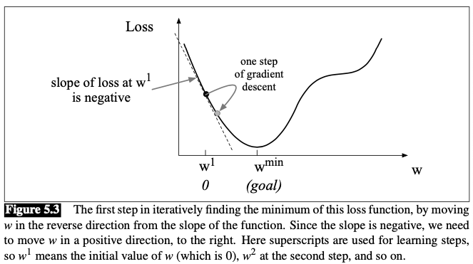
The magnitude of the amount to move in gradient descent is the value of the slope $\frac{d}{d w} f(x ; w)$ weighted by a learning rate $\eta$. A higher (faster) learning rate means that we should move w more on each step.

In the single-variable example above, The change we make in our parameter is

$$ w^{t+1}=w^{t}-\eta \frac{d}{d w} f(x ; w) $$

In $N$-dimensional space, the gradient is a vector that expresses the directinal components of the sharpest slope along each of those $N$ dimensions.

Visualizaion (E.g., $N=2$):

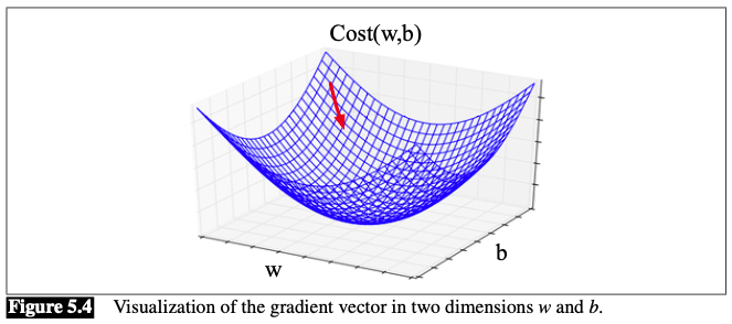
In each dimension $w_i$, we express the slope as a partial derivative $\frac{\partial}{\partial w_i}$ of the loss function. The gradient is defined as a vector of these partials:

$$ \left.\nabla_{\theta} L(f(x ; \theta), y)\right)=\left[\begin{array}{c} \frac{\partial}{\partial w_{1}} L(f(x ; \theta), y) \\ \frac{\partial}{\partial w_{2}} L(f(x ; \theta), y) \\ \vdots \\ \frac{\partial}{\partial w_{n}} L(f(x ; \theta), y) \end{array}\right] $$

Thus, the change of $\theta$ is:

$$ \theta_{t+1}=\theta_{t}-\eta \nabla L(f(x ; \theta), y) $$

The gradient for Logistic Regression

For logistic regression, the cross-entropy loss function is

$$ L_{C E}(w, b)=-[y \log \sigma(w \cdot x+b)+(1-y) \log (1-\sigma(w \cdot x+b))] $$

The derivative of this loss function is:

$$ \frac{\partial L_{C E}(w, b)}{\partial w_{j}}=[\sigma(w \cdot x+b)-y] x_{j} $$

For derivation of the derivative above we need:

• derivative of $\ln(x)$:

  $$ > \frac{d}{d x} \ln (x)=\frac{1}{x} > $$

• derivative of the sigmoid:

  $$ > \frac{d \sigma(z)}{d z}=\sigma(z)(1-\sigma(z)) > $$

• Chain rule of derivative: for $f(x)=u(v(x))$,

  $$ > \frac{d f}{d x}=\frac{d u}{d v} \cdot \frac{d v}{d x} > $$

Now compute the derivative:

$$ > \begin{aligned} > \frac{\partial L L(w, b)}{\partial w_{j}} &=\frac{\partial}{\partial w_{j}}-[y \log \sigma(w \cdot x+b)+(1-y) \log (1-\sigma(w \cdot x+b))] \\ > &=-\frac{\partial}{\partial w_{j}} y \log \sigma(w \cdot x+b) - \frac{\partial}{\partial w_{j}}(1-y) \log [1-\sigma(w \cdot x+b)] \\ > &\overset{\text{chain rule}}{=} -\frac{y}{\sigma(w \cdot x+b)} \frac{\partial}{\partial w_{j}} \sigma(w \cdot x+b)-\frac{1-y}{1-\sigma(w \cdot x+b)} \frac{\partial}{\partial w_{j}} 1-\sigma(w \cdot x+b)\\ > &= -\left[\frac{y}{\sigma(w \cdot x+b)}-\frac{1-y}{1-\sigma(w \cdot x+b)}\right] \frac{\partial}{\partial w_{j}} \sigma(w \cdot x+b) \\ > \end{aligned} > $$

Now plug in the derivative of the sigmoid, and use the chain rule one more time:

$$ > \begin{aligned} > \frac{\partial L L(w, b)}{\partial w_{j}} &=-\left[\frac{y-\sigma(w \cdot x+b)}{\sigma(w \cdot x+b)[1-\sigma(w \cdot x+b)]}\right] \sigma(w \cdot x+b)[1-\sigma(w \cdot x+b)] \frac{\partial(w \cdot x+b)}{\partial w_{j}} \\ > &=-\left[\frac{y-\sigma(w \cdot x+b)}{\sigma(w \cdot x+b)[1-\sigma(w \cdot x+b)]}\right] \sigma(w \cdot x+b)[1-\sigma(w \cdot x+b)] x_{j} \\ > &=-[y-\sigma(w \cdot x+b)] x_{j} \\ > &=[\sigma(w \cdot x+b)-y] x_{j} > \end{aligned} > $$

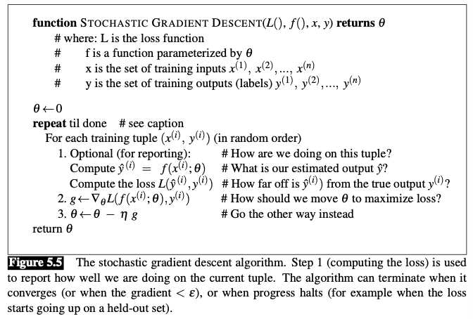
Stochastic Gradient descent

Stochastic gradient descent is an online algorithm that minimizes the loss function by

• computing its gradient after each training example, and
• nudging $\theta$ in the right direction (the opposite direction of the gradient).

The learning rate η is a (hyper-)parameter that must be adjusted.

• If it’s too high, the learner will take steps that are too large, overshooting the minimum of the loss function.
• If it’s too low, the learner will take steps that are too small, and take too long to get to the minimum.

It is common to begin the learning rate at a higher value, and then slowly decrease it, so that it is a function of the iteration $k$ of training.

Mini-batch training

Stochastic gradient descent: chooses a single random example at a time, moving the weights so as to improve performance on that single example.

• Can result in very choppy movements

Batch gradient descent: compute the gradient over the entire dataset.

• Offers a superb estimate of which direction to move the weights
• Spends a lot of time processing every single example in the training set to compute this perfect direction.

Mini-batch gradient descent

• we train on a group of $m$ examples (perhaps 512, or 1024) that is less than the whole dataset.
• Has the advantage of computational efficiency
  • The mini-batches can easily be vectorized, choosing the size of the mini-batch based on the computational resources.
  • This allows us to process all the exam- ples in one mini-batch in parallel and then accumulate the loss

Define the mini-batch version of the cross-entropy loss function (assuming the training examples are independent):

$$ \begin{aligned} \log p(\text {training labels}) &=\log \prod_{i=1} p\left(y^{(i)} | x^{(i)}\right) \\ &=\sum_{i=1}^{m} \log p\left(y^{(i)} | x^{(i)}\right) \\ &=-\sum_{i=1}^{m} L_{C E}\left(\hat{y}^{(i)}, y^{(i)}\right) \end{aligned} $$

The cost function for the mini-batch of $m$ examples is the average loss for each example:

$$ \begin{aligned} \operatorname{cost}(w, b) &=\frac{1}{m} \sum_{i=1}^{m} L_{C E}\left(\hat{y}^{(i)}, y^{(i)}\right) \\ &=-\frac{1}{m} \sum_{i=1}^{m} y^{(i)} \log \sigma\left(w \cdot x^{(i)}+b\right)+\left(1-y^{(i)}\right) \log \left(1-\sigma\left(w \cdot x^{(i)}+b\right)\right) \end{aligned} $$

The mini-batch gradient is the average of the individual gradients:

$$ \frac{\partial \operatorname{cost}(w, b)}{\partial w_{j}}=\frac{1}{m} \sum_{i=1}^{m}\left[\sigma\left(w \cdot x^{(i)}+b\right)-y^{(i)}\right] x_{j}^{(i)} $$

Regularization

🔴 There is a problem with learning weights that make the model perfectly match the training data:

• If a feature is perfectly predictive of the outcome because it happens to only occur in one class, it will be assigned a very high weight. The weights for features will attempt to perfectly fit details of the training set, in fact too perfectly, modeling noisy factors that just accidentally correlate with the class. 🤪

This problem is called overfitting.

A good model should be able to generalize well from the training data to the unseen test set, but a model that overfits will have poor generalization.

🔧 Solution: Add a regularization term $R(\theta)$ to the objective function:

$$ \hat{\theta}=\underset{\theta}{\operatorname{argmax}} \sum_{i=1}^{m} \log P\left(y^{(i)} | x^{(i)}\right)-\alpha R(\theta) $$

• $R(\theta)$: penalize large weights
  • a setting of the weights that matches the training data perfectly— but uses many weights with high values to do so—will be penalized more than a setting that matches the data a little less well, but does so using smaller weights.

Two common regularization terms:

• L2 regularization (Ridge regression)

  $$ R(\theta)=\|\theta\|_{2}^{2}=\sum_{j=1}^{n} \theta_{j}^{2} $$

  • quadratic function of the weight values

  • $\|\theta\|_{2}^{2}$: L2 Norm, is the same as the Euclidean distance of the vector $\theta$ from the origin

  • L2 regularized objective function:

    $$ \hat{\theta}=\underset{\theta}{\operatorname{argmax}}\left[\sum_{1=i}^{m} \log P\left(y^{(i)} | x^{(i)}\right)\right]-\alpha \sum_{j=1}^{n} \theta_{j}^{2} $$

• L1 regularization (Lasso regression)

  $$ R(\theta)=\|\theta\|_{1}=\sum_{i=1}^{n}\left|\theta_{i}\right| $$

  • linear function of the weight values

  • $\|\theta\|_{1}$: L1 Norm, is the sum of the absolute values of the weights.

    • Also called Manhattan distance (the Manhattan distance is the distance you’d have to walk between two points in a city with a street grid like New York)

  • L1 regularized objective function

    $$ \hat{\theta}=\underset{\theta}{\operatorname{argmax}}\left[\sum_{1=i}^{m} \log P\left(y^{(i)} | x^{(i)}\right)\right]-\alpha \sum_{j=1}^{n}\left|\theta_{j}\right| $$

L1 Vs. L2

• L2 regularization is easier to optimize because of its simple derivative (the derivative of $\theta^2$ is just $2\theta$), while L1 regularization is more complex ((the derivative of $|\theta|$ is non-continuous at zero)
• Where L2 prefers weight vectors with many small weights, L1 prefers sparse solutions with some larger weights but many more weights set to zero.
  • Thus L1 regularization leads to much sparser weight vectors (far fewer features).

Both L1 and L2 regularization have Bayesian interpretations as constraints on the prior of how weights should look.

• L1 regularization can be viewed as a Laplace prior on the weights.

• L2 regularization corresponds to assuming that weights are distributed according to a gaussian distribution with mean $μ = 0$.

  • In a gaussian or normal distribution, the further away a value is from the mean, the lower its probability (scaled by the variance $σ$)

  • By using a gaussian prior on the weights, we are saying that weights prefer to have the value 0.

    A gaussian for a weight $\theta_j$ is:

    $\frac{1}{\sqrt{2 \pi \sigma_{j}^{2}}} \exp \left(-\frac{\left(\theta_{j}-\mu_{j}\right)^{2}}{2 \sigma_{j}^{2}}\right)$

    If we multiply each weight by a gaussian prior on the weight, we are thus maximizing the following constraint:

    $$ \hat{\theta}=\underset{\theta}{\operatorname{argmax}} \prod_{i=1}^{M} P\left(y^{(i)} | x^{(i)}\right) \times \prod_{j=1}^{n} \frac{1}{\sqrt{2 \pi \sigma_{j}^{2}}} \exp \left(-\frac{\left(\theta_{j}-\mu_{j}\right)^{2}}{2 \sigma_{j}^{2}}\right) $$

    In log space, with $\mu=0$, and assuming $2\sigma^2=1$, we get:

    $$ \hat{\theta}=\underset{\theta}{\operatorname{argmax}} \sum_{i=1}^{m} \log P\left(y^{(i)} | x^{(i)}\right)-\alpha \sum_{j=1}^{n} \theta_{j}^{2} $$

Multinomial Logistic Regression

More than two classes?

Use multinomial logistic regression (also called softmax regression, or maxent classifier). The target $y$ is a variable that ranges over more than two classes; we want to know the probability of $y$ being in each potential class $c \in C, p(y=c|x)$.

We use the softmax function to compute $p(y=c|x)$:

• Takes a vector $z=[z_1, z_2,\dots, z_k]$ of $k$ arbitrary values
• Maps them to a probability distribution
  • Each value $\in (0, 1)$
  • All the values summing to $1$

For a vector $z$ of dimensionality $k$, the softmax is:

$$ \operatorname{softmax}\left(z_{i}\right)=\frac{e^{z_{i}}}{\sum_{j=1}^{k} e^{z_{j}}} \qquad 1 \leq i \leq k $$

The softmax of an input vector $z=[z_1, z_2,\dots, z_k]$ is thus:

$$ \operatorname{softmax}(z)=\left[\frac{e^{z_{1}}}{\sum_{i=1}^{k} e^{z_{i}}}, \frac{e^{z_{2}}}{\sum_{i=1}^{k} e^{z_{i}}}, \ldots, \frac{e^{z_{k}}}{\sum_{i=1}^{k} e^{z_{i}}}\right] $$

• The denominator $\sum_{j=1}^{k} e^{z_{j}}$ is used to normalize all the values into probabilities.

Like the sigmoid, the input to the softmax will be the dot product between a weight vector $w$ and an input vector $x$ (plus a bias). But now we’ll need separate weight vectors (and bias) for each of the $K$ classes.

$$ p(y=c | x)=\frac{e^{w_{c} \cdot x+b_{c}}}{\displaystyle\sum_{j=1}^{k} e^{w_{j} \cdot x+b_{j}}} $$

Features in Multinomial Logistic Regression

For multiclass classification, input features are:

• observation $x$
• candidate output class $c$

$\Rightarrow$ When we are discussing features we will use the notation $f_i(c, x)$: feature $i$ for a particular class $c$ for a given observation $x$

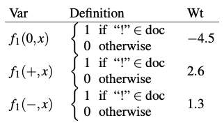
Example

Suppose we are doing text classification, and instead of binary classification our task is to assign one of the 3 classes +, −, or 0 (neutral) to a document. Now a feature related to exclamation marks might have a negative weight for 0 documents, and a positive weight for + or − documents:

Learning in Multinomial Logistic Regression

The loss function for a single example $x$ is the sum of the logs of the $K$ output classes:

$$ \begin{aligned} L_{C E}(\hat{y}, y) &=-\sum_{k=1}^{K} 1\{y=k\} \log p(y=k | x) \\ &=-\sum_{k=1}^{K} 1\{y=k\} \log \frac{e^{w_{k} \cdot x+b_{k}}}{\sum_{j=1}^{K} e^{w_{j} \cdot x+b_{j}}} \end{aligned} $$

• $1\{\}$: evaluates to $1$ if the condition in the brackets is true and to $0$ otherwise.

Gradient:

$$ \begin{aligned} \frac{\partial L_{C E}}{\partial w_{k}} &=-(1\{y=k\}-p(y=k | x)) x_{k} \\ &=-\left(1\{y=k\}-\frac{e^{w_{k} \cdot x+b_{k}}}{\sum_{j=1}^{K} e^{w_{j} \cdot x+b_{j}}}\right) x_{k} \end{aligned} $$

Reference

• Logistic Regression