Real-world Data Representation Using Tensors
import torch
Images
An image is represented as a collection of scalars arranged in a regular grid with a height and a width (in pixels).
- grayscale image: single scalar per grid point (the pixel)
- multi-color image: multiple scalars per grid point, which would typically represent different colors.
- The most common way to encode color into numbers is RGB, where a color is defined by three numbers representing the intensity of red, green, and blue.
Loading an image file
Loading a PNG image using the imageio module:
import imageio

# Assume tha PATH variable holds the path of the image
img_arr = imageio.imread(PATH)
At this point, img_arr (of shape H x W x C) is a NumPy array-like object with three dimensions:
- two spatial dimensions, height (H) and width (W)
- a third dimension corresponding to the red, green, and blue channels (C)
Change the layout to PyTorch supported layout
PyTorch modules dealing with image data require tensors to be laid out as C × H × W : channels, height, and width, respectively.
We can use the tensor’s permute method with the old dimensions for each new dimension to get to an appropriate layout. Given an input tensor H × W × C as obtained previously, we get a proper layout by having channel 2 first and then channels 0 and 1:
img = torch.from_numpy(img_arr) # np arr -> torch tensor
out = img.permute(2, 0, 1) # adjust to pytorch required layout
permute() operation does NOT make a copy of the tensor data. Instead, out uses the same underlying storage as img and only plays with the size and stride information at the tensor level.Create a dataset of multiple images
To create a dataset of multiple images to use as an input for our neural networks, we store the images in a batch along the first dimension to obtain an N × C × H × W tensor.
How to do this?
Pre-allocate a tensor of appropriate size.
batch = torch.zeros(batch_size, 3, 256, 256, dtype=torch.uint8)dtype=torch.uint8: we’re expecting each color to be represented as an 8-bit integer, as in most photographic formats from standard consumer cameras.
Fill it with images loaded from a directory
Now we can load all PNG images from an input directory and store them in the tensor:
import os

# assume data_dir is our input directory
filenames = [name for name in os.listdir(data_dir)
                if os.path.splitext(name)[-1] == '.png']

for i, filename in enumerate(filenames):
    img_arr = imageio.imread(os.path.join(data_dir, filename))
    img_t = torch.from_numpy(img_arr)
    img_t = img_t.permute(2, 0, 1)
    img_t = img_t[:3] # just keep the first three channels (RGB)
    batch[i] = img_t
Normalizing the data
Neural networks exhibit the best training performance when the input data ranges roughly from 0 to 1, or from -1 to 1.
So a typical thing we’ll want to do is
Cast a tensor to floating-point
Normalize the values of the pixels
It depends on what range of the input we decide should lie between 0 and 1 (or -1 and 1)
One possibility is to just divide the values of the pixels by 255 (the maximum representable number in 8-bit unsigned)
batch = batch.float() # cast to floating point tensor
batch /= 255.0 # normalize
Another possibility for normalization is to compute the mean and standard deviation of the input data and scale it so that the output has zero mean and unit standard deviation across each channel:
$$ \forall x \in \text{dataset}: \quad x:= \frac{x - \text{mean}}{\text{standard deviation}} $$n_channels = batch.shape[1] # shpae is: N x C x H x W for c in range(n_channels): mean = torch.mean(batch[:, c]) std = torch.std(batch[:, c]) batch[:, c] = (batch[:, c] - mean) / std
Tabular data
Spreadsheet, CSV file, or database: a table containing one row per sample (or record), where columns contain one piece of information about our sample.
- There’s no meaning to the order in which samples appear in the table (sch a table is a collection of independent samples)
- Tabular data is typically not homogeneous: different columns don’t have the same type.
PyTorch tensors, on the other hand, are homogeneous. Information in PyTorch is typically encoded as a number, typically floating-point (though integer types and Boolean are supported as well).
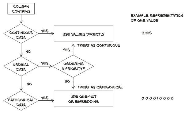
Continuous, ordinal, and categorical values
| Type of values | Have order? | Have numerical meaning? |
|---|---|---|
| categorical | ❌ | ❌ |
| ordinal | ❌ | ✅ |
| continuous | ✅ | ✅ |
continuous values
strictly ordered
a difference between various values has a strict meaning
Example
Stating that package A is 2 kilograms heavier than package B, or that package B came from 100 miles farther away than A has a fixed meaning, regardless of whether package A is 3 kilograms or 10, or if B came from 200 miles away or 2,000.
The literature actually divides continuous values further
- ratio scale: it makes sense to say something is twice as heavy or three times farther away
- interval scale: The time of day, does have the notion of difference, but it is not reasonable to claim that 6:00 is twice as late as 3:00
ordinal values
The strict ordering we have with continuous values remains, but the fixed relationship between values no longer applies.
Example:
Ordering a small, medium, or large drink, with small mapped to the value 1, medium 2, and large 3. The large drink is bigger than the medium, in the same way that 3 is bigger than 2, but it doesn’t tell us anything about how much bigger.
If we were to convert our 1, 2, and 3 to the actual volumes (say, 8, 12, and 24 fluid ounces), then they would switch to being interval values.
We can’t “do math” on the values outside of ordering them (trying to average large = 3 and small = 1 does not result in a medium drink!)
categorical values
have neither ordering nor numerical meaning to their values. These are often just enumerations of possibilities assigned arbitrary numbers.
Example
Assigning water to 1, coffee to 2, soda to 3, and milk to 4. There’s no real logic to placing water first and milk last; they simply need distinct values to dif- ferentiate them. We could assign coffee to 10 and milk to –3, and there would be no significant change
Loading tabular data
Python offers several options for quickly loading a CSV file. Three popular options are
- The
csvmodule that ships with Python - NumPy
- Pandas (most time- and memory-efficient)
Since PyTorch has excellent NumPy interoperability, we’ll go with that.
import csv

# assume PATH variable holds the csv file
tabular_data_numpy = np.loadtxt(PATH,
                         dtype=np.float32, # type of the np arr should be
                         delimiter=";", # delimiter used to separate values in each orw
                         skiprows=1 # the first line should not be read since it contains the col names
                         )
Convert the numpy array to pytorch tensor:
tabular_data_tensor = torch.from_numpy(tabular_data_numpy)
Get the names of each column
col_list = next(csv.reader(open(PATH), delimiter=';'))
One-hot encoding
Assume that we use 1 to 10 to represent the score/class. We could build a one-hot encoding of the scores: encode each of the 10 scores in a vector of 10 elements, with all elements set to 0 but one, at a different index for each score. For example, a score of 1 could be mapped onto the vector (1,0,0,0,0,0,0,0,0,0), a score of 5 onto (0,0,0,0,1,0,0,0,0,0), and so on. Note that there’s no implied ordering or distance (i.e. they are categorical values) when we use one-hot encoding.
We can achieve one-hot encoding using the scatter_ method, which fills the tensor with values from a source tensor along the indices provided as arguments:
# assume that we already have the score tensor
score
tensor([6, 6, ..., 7, 6])
score.shape
torch.Size([4898])
score_onehot = torch.zeros(score.shape[0], 10) # in our case: score.shape[0] = 4898
score_onehot.scatter_(1, score.unsqueeze(1), 1.0)
scatter_(dim, index, src)
dim: The dimension along which the following two arguments are specified
index: A column tensor indicating the indices of the elements to scatter
required to have the same number of dimensions as the tensor we scatter into.
Since
score_onehothas two dimensions (4,898 × 10), we need to add an extra dummy dimension toscoreusingunsqueeze
src: A tensor containing the elements to scatter or a single scalar to scatter (1, inthis case)
In other words, the previous invocation reads, “For each row, take the index of the score label (which coincides with the score in our case) and use it as the column index to set the value 1.0.” The end result is a tensor encoding categorical information.
When to categorise?
- Categorical: losing the ordering part, and hoping that maybe our model will pick it up during train- ing if we only have a few categories
- Continuous: introducing an arbitrary notion of distance
Text
🎯 Goal: turn text into tensors of numbers that a neural network can process.
Converting text to numbers
There are two particularly intuitive levels at which networks operate on text:
- character level: processing one character at a time
- word level: individual words are the finest-grained entities to be seen by the network.
The technique with which we encode text information into tensor form is the same whether we operate at the character level or the word level.
One-hot-encoding characters
First we will load the text:
# assume PATH variable holds the txt file
with open(PATH, encoding='utf8') as f:
    text = f.read()
Encoding of the character: Every written character is represented by a code (a sequence of bits of appropriate length so that each character can be uniquely identified).
We are going to one-hot encode our characters. Depending on the task at hand, we could
- make all of the characters lowercase, to reduce the number of different characters in our encoding
- screen out punctuation, numbers, or other characters that aren’t relevant to our expected kinds of text.
At this point, we need to parse through the characters in the text and provide a one-hot encoding for each of them: Each character will be represented by a vector of length equal to the number of different characters in the encoding. This vector will contain all zeros except a one at the index corresponding to the location of the character in the encoding.
For the sake of simplicity, we first split our text into a list of lines and pick an arbitrary line to focus on:
lines = text.split('\n') # split text into a list of lines
line = lines[200] # pick arbitrary line

letter_t = torch.zeros(len(line), 128) # 128 hardcoded due to the limits of ASCII

for i, letter in enumerate(line.lower().strip()):
    # The text uses directional double quotes, which are not valid ASCII,
    # so we screen them out here.
    letter_index = ord(letter) if ord(letter) < 128 else 0
    letter_t[i][letter_index] = 1
One-hot encoding whole words
We’ll define a helper functionclean_words, which takes text and returns it in lowercase and stripped of punctuation.
def clean_words(input_str):
    punctuation = '.,;:"!?”“_-'
    word_list = input_str.lower().replace('\n', '').split()
    word_list = [word.strip(punctuation) for word in word_list]
    return word_list
When we call it on our “Impossible, Mr. Bennet” line, we get the following:
words_in_line = clean_words(line)
line, words_in_line
('“Impossible, Mr. Bennet, impossible, when I am not acquainted with him',
 ['impossible',
  'mr',
  'bennet',
  'impossible',
  'when',
  'i',
  'am',
  'not',
  'acquainted',
  'with',
  'him'])
Now, let’s build a mapping of all words in text to indexes in our encoding:
word_list = sorted(set(clean_words(text)))
word2index_dict = {word: i for (i, word) in enumerate(word_list)}
word2index_dict is now a dictionary with words as keys and an integer as a value. We will use it to efficiently find the index of a word as we one-hot encode it. For example, let’s look up the index of word “possible”:
word2index_dict['possible']
10421
Let’s see how can we one-hot encode the words of sentence “Impossible, Mr. Bennet, impossible, when I am not acquainted with him”:
- create an empty tensor
- assign the one-hot-encoded values of the word in the sentence
# create an empty tensor
word_t = torch.zeros(len(words_in_line), len(word2index_dict))

# assign the one-hot-encoded values of the word in the sentence
for i, word in enumerate(words_in_line):
    word_index = word2index_dict[word]
    word_t[i][word_index] = 1
    print(f"{i:2} {word_index:4} {word}")
 0 6925 impossible
 1 8832 mr
 2 1906 bennet
 3 6925 impossible
 4 14844 when
 5 6769 i
 6  714 am
 7 9198 not
 8  312 acquainted
 9 15085 with
10 6387 him
word_t.shape
torch.Size([11, 15514])
The choice between character-level and word-level encoding leaves us to make a trade-off
- In many languages, there are significantly fewer characters than words: representing characters has us representing just a few classes, while representing words requires us to represent a very large number of classes
- On the other hand, words convey much more meaning than individual characters, so a representation of words is considerably more informative by itself.
Text embeddings
Embedding is to find an effective way to map individual words into a fixed number (let’s say, 100) dimensional space in a way that facilitates downstream learning. An ideal solution would be to generate the embedding in such a way that words used in similar contexts mapped to nearby regions of the embedding.
Embeddings are often generated using neural networks, trying to predict a word from nearby words (the context) in a sentence. In this case, we could start from one-hot-encoded words and use a (usually rather shallow) neural network to generate the embedding. Once the embedding was available, we could use it for downstream tasks.
One interesting aspect of the resulting embeddings is that similar words end up not only clustered together, but also having consistent spatial relationships with other words. For example, if we were to take the embedding vector for apple and begin to add and subtract the vectors for other words, we could begin to perform analogies like apple - red - sweet + yellow + sour and end up with a vector very similar to the one for lemon.