Using Neural Network to Fit Data

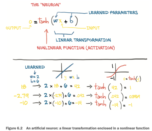
Artficial neurons

Core of deep learning are neural networks: mathematical entities capable of representing complicated functions through a composition of simpler functions.

The basic building block of these complicated functions is the neuron

• At its core, it is nothing but a linear transformation of the input (for example, multiplying the input by a number [the weight] and adding a constant [the bias]) followed by the application of a fixed nonlinear function (referred to as the activation function).
• Mathematically, we can write this out as o = f(w * x + b), with x as our input, w our weight or scaling factor, and b as our bias or offset. f is our activation function, set to the hyperbolic tangent, or tanh function here.

Composing a multilayer network

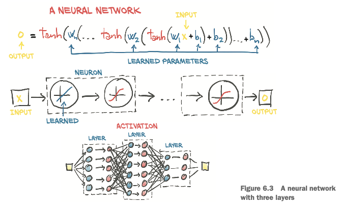
is made up of a composition of functions like those we just discussed

x_1 = f(w_0 * x + b_0) 
x_2 = f(w_1 * x_1 + b_1) 
...
y = f(w_n * x_n + b_n)

where the output of a layer of neurons is used as an input for the following layer.

The error function

• Neural networks do not have property of a convex error surface
• There’s no single right answer for each parameter we’re attempting to approximate. Instead, we are trying to get all of the parameters, when acting in concert, to produce a useful output.
• Since that useful output is only going to approximate the truth, there will be some level of imperfection. Where and how imperfections manifest is somewhat arbitrary, and by implication the parameters that control the output (and, hence, the imperfections) are somewhat arbitrary as well. 🤪

Activation functions

The simplest unit in (deep) neural networks is a linear operation (scaling + offset) followed by an activation function. The activation function plays two important roles:

• In the inner parts of the model, it allows the output function to have different slopes at different values—something a linear function by definition cannot do. By trickily composing these differently sloped parts for many outputs, neural networks can approximate arbitrary functions
• At the last layer of the network, it has the role of concentrating the outputs of the preceding linear operation into a given range.
  • Capping the output range
  • Compressing the output range

Some activation functions:

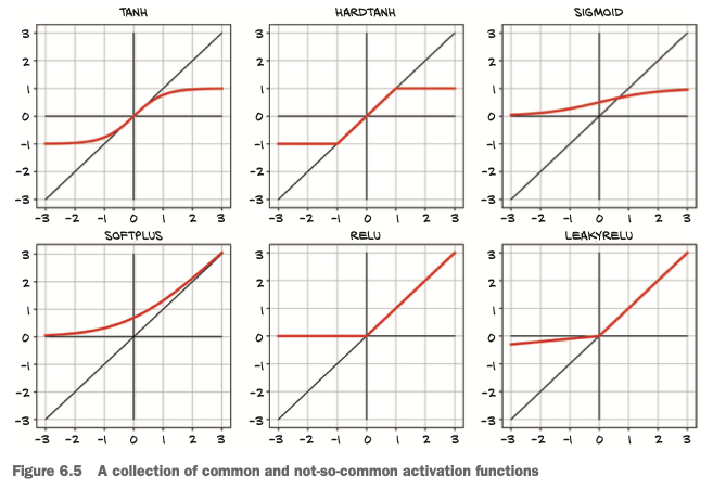
ReLU (Rectified Linear Unit) is currently considered one of the best-performing general activation functions. The LeakyReLU function modifies the standard ReLU to have a small positive slope, rather than being strictly zero for negative inputs (typically this slope is 0.01, but it’s shown here with slope 0.1 for clarity).

Choosing the best activation function

By definition, activation functions are

• nonlinear: The nonlinearity allows the overall network to approximate more complex functions.
• differentiable: so that gradients can be computed through them.

The following are true for the functions:

• They have at least one sensitive range, where nontrivial changes to the input result in a corresponding nontrivial change to the output. This is needed for training.
• Many of them have an insensitive (or saturated) range, where changes to the input result in little or no change to the output.

Often (but far from universally so), the activation function will have at least one of these:

• A lower bound that is approached (or met) as the input goes to negative infinity
• A similar-but-inverse upper bound for positive infinity

🤔 What learning means for a neural network

Building models out of stacks of linear transformations followed by differentiable activations leads to models that can approximate highly nonlinear processes and whose parameters we can estimate surprisingly well through gradient descent, even when dealing with models with millions of parameters. What makes using deep neural networks so attractive is that it saves us from worrying too much about the exact function that represents our data. With a deep neural network model, we have a universal approximator and a method to estimate its parameters. 👏

Training consists of finding acceptable values for these weights and biases so that the resulting network correctly carries out a task. By carrying out a task successfully, we mean obtaining a correct output on unseen data produced by the same data-generating process used for training data. A successfully trained network, through the values of its weights and biases, will capture the inherent structure of the data in the form of meaningful numerical representations that work correctly for previously unseen data.

Deep neural networks give us the ability to approximate highly nonlinear phenomena without having an explicit model for them. Instead, starting from a generic, untrained model, we specialize it on a task by providing it with a set of inputs and outputs and a loss function from which to backpropagate. Specializing a generic model to a task using examples is what we refer to as learning, because the model wasn’t built with that specific task in mind—no rules describing how that task worked were encoded in the model.

The PyTorch nn module

torch.nn

• submodule dedicated to neural networks
• contains the building blocks needed to create all sorts of neural network architectures. Those building blocks are called modules in PyTorch parlance (such building blocks are often referred to as layers in other frameworks).

A module

• can have one or more Parameter instances as attributes, which are tensors whose values are optimized during the training process
• can also have one or more submodules (subclasses of nn.Module) as attributes, and it will be able to track their parameters as well.

Using __call__ rather than forward

• All PyTorch-provided subclasses of nn.Module have their __call__ method defined. This allows us to instantiate an nn.Linear and call it as if it was a function.
• From user code, we should not call forward directyly

y = model(x) # correct
y = model.forward(x) # Don't do it!

Dealing with batches

PyTorch nn.Module and its subclasses are designed to do so on multiple samples at the same time.

• Modules expect the zeroth dimension of the input to be the number of samples in the batch.
• E.g, we can create an input tensor of size B × Nin, where
  • B: the size of the batch
  • Nin: the number of input features

Loss functions

Loss functions in nn are still subclasses of nn.Module, so we will create an instance and call it as a function.

Our training loop looks like this:

def training_loop(n_epochs, optimizer, model, loss_fn, t_u_train, t_u_val,
                  t_c_train, t_c_val):
    for epoch in range(1, n_epochs+1):
        
        # forward pass in training set
        t_p_train = model(t_u_train) 
        loss_train = loss_fn(t_p_train, t_c_train)

        # forward pass in validation set
        with torch.no_grad():
            t_p_val = model(t_u_val)
            loss_val = loss_fn(t_p_val, t_c_val)

        optimizer.zero_grad()
        loss_train.backward()
        optimizer.step()

        if epoch == 1 or epoch % 1000 == 0:
            print(f"Epoch {epoch}, Training loss {loss_train.item():.4f},"
            f" Validation loss {loss_val.item():.4f}")

, and we want to use Mean Square Error (MSE) as our loss function:

linear_model = nn.Linear(1, 1)
optimizer = optim.SGD(linear_model.parameters(), lr=1e-2)

training_loop(n_epochs=3000, optimizer=optimizer, model=linear_model,
              loss_fn=nn.MSELoss(), t_u_train=t_un_train, t_u_val=t_un_val,
              t_c_train=t_c_train, t_c_val=t_c_val)

Building neural networks using PyTorch

nn.Sequential container

nn provides a simple way to concatenate modules through the nn.Sequential container. For example, let’s build the simplest possible neural network: a linear module, followed by an activation function, feeding into another linear module.

seq_model = nn.Sequential(nn.Linear(1, 13), # 1 input feature to 13 hidden features
                          nn.Tanh(), # pass them through a tanh activation
                          nn.Linear(13, 1)) # linearly combine the resulting 13 numbers into 1 output feature

seq_model

Sequential(
  (0): Linear(in_features=1, out_features=13, bias=True)
  (1): Tanh()
  (2): Linear(in_features=13, out_features=1, bias=True)
)

Inspecting parameters

Calling model.parameters() will collect weight and bias from both the first and second linear modules. It’s instructive to inspect the parameters in this case by printing their shapes:

[param.shape for param in seq_model.parameters()]

[torch.Size([13, 1]), torch.Size([13]), torch.Size([1, 13]), torch.Size([1])]

We can also use named_parameters to identify parameters by name:

for name, param in seq_model.named_parameters():
    print(f"{name}: {param.shape}")

0.weight: torch.Size([13, 1])
0.bias: torch.Size([13])
2.weight: torch.Size([1, 13])
2.bias: torch.Size([1])

Sequential also accepts an OrderedDict, in which we can name each module passed to Sequential:

from collections import OrderedDict

seq_model = nn.Sequential(OrderedDict([('hidden_linear', nn.Linear(1, 8)),
                                       ('hidden_activation', nn.Tanh()),
                                       ('output_linear', nn.Linear(8, 1))]))

seq_model

Sequential(
  (hidden_linear): Linear(in_features=1, out_features=8, bias=True)
  (hidden_activation): Tanh()
  (output_linear): Linear(in_features=8, out_features=1, bias=True)
)

for name, param in seq_model.named_parameters():
    print(f"{name}: {param.shape}")

hidden_linear.weight: torch.Size([8, 1])
hidden_linear.bias: torch.Size([8])
output_linear.weight: torch.Size([1, 8])
output_linear.bias: torch.Size([1])

We can also access a particular Parameter by using submodules as attributes:

seq_model.output_linear.bias

Parameter containing:
tensor([-0.0328], requires_grad=True)